|
Particle location and tracking tutorial |
| Home | Tutorial | Code | |
Step 1: Location of particle positions
|
Ok,
so you have worked really hard to get nice images of whatever particles
you would like to locate and eventually track. The images can be in any
format recognized by Matlab (.jpg, .tif, etc.), but the features you wish to
locate need to be well-resolved and compatible with the algorithms
employed here. As a rule of thumb, you should be able to
locate most blobs discernable by eye.
|
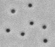
| Here is an image of some colloidal particles viewed in bright field. To read, display, and query this image out some, type the following at the matlab prompt. | |||||||||||||||||||||||||||||||
 |
>> a =
double(imread('test.jpg'));
|
||||||||||||||||||||||||||||||
| The image above is perfect for locating, however the particles must be bright compared to the background for the locating to work properly. If your images look like those above do the following. If they already look bright on dark skip this step. | |
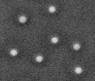 |
>> a =
255-a; |
| Now it's time to use a macro. The first thing to do is spatially filter the image. To accomplish this type the following. | |||||||||||||||||||||||||||||||
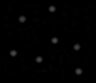 |
>> b =
bpass(a,1,10); |
||||||||||||||||||||||||||||||
|
bpass is a spatial bandpass filter which smooths the image and subtracts the background off. The two numbers are the spatial wavelength cutoffs in pixels. The first one is almost always '1'. The second number should be something like the diameter of the 'blob's you want to find in pixels. Try a few values and use the one that gives you nice, sharply peaked circular blobs where your particles were; remember the numbers you used for bpass. The next step is to identify the blobs that bpass has found as features. You will want to first use the pkfnd macro. >> pk = pkfnd(b,60,11); This
should give you the location of all of the peaks that are above the
given threshold value here given by 60. This number will depend on how
your final band-passed image looks. One way to roughly estimate the
brightest feature is to do the following.
The second parameter (set to 11) is roughly the diameter of the average feature to look for in pixels. This parameter is helpful for noisy data. If you have noisy data, read the preamble in pkfnd. As with all of this code, make sure that you read the complete documentation. The variable pk
provides a first estimate of particle locations to pixel-level
accuracy. You can get a more accurate and precise estimate of
the particle location by calculating the centroid of each blob...
That's basically it! You have just successfully located, or pre-tracked a single image. Don't you feel awesome! Now you that you have done one, you can do them all. You need to understand little more than a for loop to make this work Also, making sure that you have found your features to sub-pixel accuracy, please refer to the IDL tutorial. The commands to check for sub-pixel feature location are quite simple and can be implemented in a single matlab line given below. >> hist(mod(cnt(:,1),1),20); This will result in a histogram of the x-positions modulo 1, which should look flat if you have enough features and they are not single pixel biased. |
|||||||||||||||||||||||||||||||
Step 2: Linking particle locations to form trajectories
|
Now comes the really fun part. If you have successfully generated a set of files that contains the x,y and even z positions of your data, then you can track the particle positions over time. If you have done this in IDL, then the conversion to Matlab should be very straight forward, as the macro is exactly a replica of the IDL version. First thing you
should do is read the documentation on track. It is
essential that you put your position list in the required format. Once
you have that, you are in the clear. Just invoke track with the
parameters that are right for you and you should be fine. Here is an
example of what to do. >> tr = track(pos_lst, 3); Here, pos_lst
is the list of particle positions and the timestamp for each frame to
be considered concatenated vertically. By passing an additional
structure, param, in the function call, you can tweak the important
parameters used in tracking:
>>
help track <>Good luck! |