Hydrogen Hamiltonian

The hydrogen atom Hamiltonian is

\[\hat{H}=\frac{\hat{p}_{x}^{2}+\hat{p}_{y}^{2}+\hat{p}_{z}^{2}}{2 \mu}-\frac{e^{2}}{\hat{r}} \quad \text{with}\quad \mu=\frac{m_{e} m_{N}}{m_{0}+m_{N}}=\text { reduced mass }.\]

Recall that the kinetic energy can be decomposed into its radial and angular pieces via \[\hat{H}=\frac{\hat{p}_{r}^{2}}{2 \mu}+\frac{\mathbf{L}^{2}}{2 \mu \hat{r}^{2}}-\frac{e^{2}}{\hat{r}}\] We are using cgs units here, which is common in atomic physics. Note how \(\hat{H}\) commutes with \(\hat{\mathbf{L}}^{2}\) and \(\hat{L}_{z}\), because \(\hat{\mathbf{p}}\) is a vector operator as is \(\hat{\mathbf{r}}\) and this is a function of \(\hat{p}^{2}\) and \(\hat{r}^{2}\) only. This means we can simultaneously diagonalize \(\hat{H} , \hat{\mathbf{L}}^{2}\) and \(\hat{L}_{z} \Rightarrow|\psi\rangle=\left|\psi_{r}\right\rangle \otimes\left|l, m\right\rangle\). This is because we know that the eigenstates of \(\hat{\mathbf{L}}^{2}\) and \(\hat{L}_{z} \text{ are } \left|l, m\right\rangle\)

If we operate \(\hat{H}\) on \(|\psi\rangle\) then since \(\hat{\mathbf{L}}^{2}\mid l, m\rangle=\) \(\hbar^{2} l(l +1)\mid l, m \rangle\), we have \[\hat{H}_{l}\left|\psi_{r}\right\rangle=E\left|\psi_{r}\right\rangle~~\text{with}~~ \hat{H}_{l}=\frac{\hat{p}_{r}^{2}}{2 \mu}+\frac{\hbar^{2} l(l+1)}{2 \mu \hat{r}^{2}}-\frac{e^{2}}{\hat{r}}\] which is the Hamiltonian for angular momentum \(l\).

Factorization

Our job is to factorize each of these \(\hat{H}_{l}\) Hamiltonians and find all of their eigenvalues. There are two ways do this and use will use a shortcut solution here. You will use the standard Schrödinger method in the homework.

With a little thought, we realize we should try \[\hat{B}_{r}(l)=\frac{1}{\sqrt{2 \mu}}\left(\hat{p}_{r}-i \hbar\left(\frac{\alpha}{a_{0}}+\frac{\beta}{\hat{r}}\right)\right)\] with \(\alpha\) and \(\beta\) dimensionless numbers, and \(a_{0}=\frac{\hbar^{2}}{\mu e^{2}}=\) Bohr radius \(=0.529\) Å.

The choice of "constant + \(\frac{1}{\hat{r}}\)" fforthe superpotential is governed by the fact that the square of it plus the commutator with \(\hat{p}_{r}\) includes constant, \(\frac{1}{\hat{r}}\) and \(\frac{1}{\hat{r}^{2}}\) terms. This is just what we need to be able to factorize the Hamiltonian.

We compute \[\begin{aligned} \hat{B}_{r}^{\dagger}(l) \hat{B}_{r}(l)= & \frac{\hat{p}_{r}^{2}}{2 \mu}-\frac{i \hbar}{2 \mu}\left[\hat{p}_{r}, \frac{\alpha}{a_{0}}+\frac{\beta}{\hat{r}}\right] +\frac{\hbar^{2}}{2 \mu}\left[\frac{\alpha}{a_{0}}+\frac{\beta}{\hat{r}}\right]^{2} \end{aligned}\] Recall that \(\left[\hat{p}_{r}, \hat{r}\right]=-i \hbar\) and \(\left[\hat{p}_{r}, \frac{1}{\hat{r}}\right]=\frac{i \hbar}{\hat{r}^{2}}\). Then, we have \[\hat{B}_{r}^{\dagger}(l) \hat{B}_{r}(l)=\frac{\hat{p}_{r}^{2}}{2 \mu}+\frac{\hbar^{2}}{2 \mu \hat{r}^{2}}\left(\beta+\beta^{2}\right)+\frac{\hbar^{2}}{\mu} \frac{\alpha \beta}{a_{0} \hat{r}}+\frac{\hbar^{2}}{2 \mu} \frac{\alpha^{2}}{a_{0}^{2}}.\] This implies that \[\beta(\beta+1)=l(l+1), \quad \alpha \beta=-1 \quad\text{and}\quad \tilde{E}_{l}=-\frac{\hbar^{2} \alpha^{2}}{2 \mu a_{0}^{2}},\] which we use to make the rest of the notation easier. So \(\beta=l\) or \(\beta=-l-1\), \(\alpha=-\frac{1}{\beta}\) and \(\tilde{E}_{l}=-\frac{1}{2} \frac{1}{a_{0}} \frac{e^{2}}{\beta^{2}}\). This then implies that \(\tilde{E}_{l}=-\frac{1}{2} \frac{e^{2}}{a_{0}} \frac{1}{l^{2}}\) or \(-\frac{1}{2} \frac{e^{2}}{a_{0}} \frac{1}{(l+1)^{2}}\)
Our rule is to choose \(\beta=-l-1\), which then requires \(\alpha=\frac{1}{l+1}\), so that we have \(W(r)>0 \text{ as } r \rightarrow \infty\). The other choice will give us the wrong sign.

Hence, we have \[\begin{aligned} \hat{B}_{r}(l) & =\frac{1}{\sqrt{2m}}\left[\hat{p}_{r}-i \hbar\left(\frac{1}{a_{0}(l+1)}-\frac{l +1}{\hat{r}}\right)\right] ~~ \text { and }~~ \hat{H}_{l} =\hat{B}_{r}^{\dagger}(l) \hat{B}_{r}(l)+\tilde{E}_{l}. \end{aligned}\]

Intertwining

Next is intertwining: First we compute the opposite order of the product of the ladder operators \[\begin{aligned} \hat{B}_{r}(l) \hat{B}_{r}^{\dagger} (l) & =\frac{1}{2 \mu}\left[\hat{p}_{r}^{2}-i \hbar\left[\hat{P}_{r}, \frac{l+1}{\hat{r}}\right]+\hbar^{2}\left(\frac{1}{a_{0}^{2}(l+1)^{2}}-\frac{1}{a_{0} \hat{r}^{2}}+\frac{(l+1)}{\hat{r}^{2}}\right)\right] \\ & =\frac{\hat{p}_{r}^{2}}{2 \mu}+\frac{\hbar^{2}(l+1)(l+2)}{2 \mu \hat{r}^{2}}-\frac{e^{2}}{\hat{r}}+\frac{e^{2}}{2 a_{0}(l+1)^{2}} \\ & =\hat{H}_{l+1}-\tilde{E}_{l}. \end{aligned}\] So, we have that \[\begin{aligned} \hat{H}_{l} \hat{B}_{r}^{\dagger}(l) & =\left(\hat{B}_{r}^{\dagger}(l) \hat{B}_{r}(l)+\tilde{E}_{l}\right) \hat{B}_{r}^{\dagger}(l) \\ & =\hat{B}_{r}^{\dagger}(l)\left(\hat{B}_{r}(l) \hat{B}_{r}^{\dagger}(l)+\tilde{E}_{l}\right) \\ & =\hat{B}_{r}^{\dagger}(l) \hat{H}_{l+1}. \end{aligned}\]

Energy eigenstates

We use these results to construct the energy eigenstates. We label the energies with \(n=l+1\) \[E_{n}=-\frac{e^{2}}{2 a_{0} n^{2}}=\tilde{E}_{l{=}n+1}\] The first state we work with, which is the ground state of \(\hat{H}_{l}\), is obviously \[\hat{B}_{r}(l)|n{=}l+1, l\rangle=0,\] with energy \(E_{n}=-\frac{e^{2}}{2 a_{0}(l+1)^{2}}\) because of the positive-semidefinite form of the Hamiltonian (note that the index satisfies \(n=l+1\)). Hence, \[\hat{B}_{r}(n-1)|n, l{=}n-1\rangle=0 \quad \text{and}\quad E_{n}=-\frac{e^{2}}{2 a_{0} n^{2}}.\]

The claim is the state \[|n l\rangle=\hat{B}_{r}^{\dagger}(l) \hat{B}_{r}^{\dagger}(l + 1) \cdots \hat{B}_{r}^{\dagger}(n-2)\left|n , l{=}n-1\right\rangle\] is an eigenstate of \(\hat{H}_{l}\) with energy \(E_{n}=-\frac{e^{2}}{2 a_{0}n^{2}}\). We verify with intertwining: \[\begin{aligned} & \hat{H}_{l} \mid n l\rangle=\underbrace{\hat{H}_{l} \hat{B}_{r}^{\dagger}(l)}_{\text{intertwining}} \hat{B}_{r}^{\dagger}(l +1) \cdots \hat{B}_{r}^{\dagger}(n-2) \mid n, l=n-1\rangle \\ & =\hat{B}_{r}^{\dagger}(l) \hat{H}_{l+1}{ \hat{B}^{\dagger}_{r}(l-1)} \cdot {\hat{B}^{\dagger} r} {(n-2)}\left|n, l=n-1\right\rangle \\ & =\hat{B}_{r}^{\dagger}(l) \hat{B}_{r}^{\dagger}(l +1) \cdots \hat{B}_{r}^{\dagger}(n-2) \hat{H}_{n-1}|n, l=n-1\rangle \\ & =E_{n} \hat{B}_{r}^{\dagger}(l) \hat{B}_{r}^{\dagger}(l+1) \cdots \hat{B}_{r}^{\dagger}(n-2)|n, l=n-1\rangle \\ & =E_{n}|n, l\rangle. \end{aligned}\] So, it is an eigenstate as claimed.
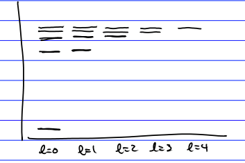
Note, we have found a chain of states with \(0 \leq l \leq n-1\) that all have energy \(E_{n}\)

The spectrum lis shown in the figure.

Energy wavefunctions

Our next step is to find the wavefunction. Although it might not seem like it, the string of \(\hat{B}_{r}\) operators multiplying \(|n, l{=}n-1\rangle\) is a polynomial in \({\hat{\mathbf{r}}}\). We see this when we notice that the condition \[\hat{B}_{r}(n-1)\mid n, l{=}n-1\rangle=0\] can be rewritten as \[\hat{p}_{r}\left|n , l{=}n-1\right\rangle=i \hbar\left(\frac{1}{n a_{0}}-\frac{n}{\hat{r}}\right)|n, l{=}n-1\rangle.\] This means the \(\hat{p}_{r}\)’s in the string of \(\hat{B}_r^{\dagger}\)’s become polynomials in \(\frac{1}{\hat{r}}\). We need to determine how to find their form. Obviously, we need to use induction.

To organize the work, we need to establish some notation, which, like in the SHO, uses the 20-20 hindsight with respect to the final answer, so everything is neat. We have \[\begin{aligned} |n l\rangle= & \hat{B}_{r}^{\dagger}(l) \hat{B}_{r}^{\dagger}(l+1) \cdots \hat{B}_{r}^{\dagger}(n-2) \mid n, l{=}n-1\rangle \\ = & \left(\frac{-i \hbar}{\sqrt{2 \mu } n a_{0}}\right)^{n-l-1}\left(\frac{n a_{0}}{2 \hat{r}}\right)^{n-l-1} \frac{(2 n-1)!}{(n+l)!} \frac{(n-l-1)!l!}{(n-1)!} L_{n-l-1}^{2 l+1}\left(\frac{2 \hat{r}}{n a_{0}}\right)|n, l{=}n-1\rangle, \end{aligned}\] which defines our polynomial operator \(L_{n-l-1}^{2 l+1}\left(\frac{2 \hat{r}}{n a_{0}}\right)\). The index \(n-l-1\) appears because that is how many \(\hat{B}_{r}^{\dagger}\) operators we have. The factorials are used to put the result in "standard" form. We write \(L_{n-l -1}^{2 l + 1}\left(\frac{2 \hat{r}}{n a_{0}}\right)=\sum_{j=0}^{n-l-1} a_{j}^{2 l+1}\left(\frac{2 \hat{r}}{n a_{0}}\right)^{j}\).

Recurrence relation

To find the recurrence relation, we de the same as with the SHO and we factor off a \(\hat{B}_{r}^{\dagger}(l)\) from the left to give us \[\begin{aligned} & \left(\frac{-i \hbar}{\sqrt{2 \mu } n a_0} \right)^{n-l-1}\left(\frac{n a_{0}}{2 \hat{r}}\right)^{n-l-1} \frac{(2 n-1)!}{(n+l)!} \frac{(n-l-1)!l!}{(n-1)!} \sum_{j=0}^{n-l-1} a_{j}^{2 l+1}\left(\frac{2 \hat{r}}{n a_{0}}\right)^{j}\left|n, l{=}n-1\right\rangle \\ = & \left(\frac{-i \hbar}{\sqrt{2 \mu } n a_0}\right)^{n-l-2} \frac{(2 n-1)!}{(n+l-1)!} \frac{(n-l-2)!(l+1)!}{(n-1)!} \hat{B}^{\dagger}_r(l)\left(\frac{n a_{0}}{2 \hat{r}}\right)^{n-l-2} \sum_{j=0}^{n-l-2} a_{j}^{2 l+3}\left(\frac{2 \hat{r}}{n a_{0}}\right)^{j} \mid n ,l{=}n-1\rangle. \end{aligned}\] Compute \[\begin{aligned} &\hat{B}_{r}^{\dagger}(l)\left(\frac{2 \hat{r}}{n_{0}}\right)^{n -l-2-j}\left|n, l{=}n-1\right\rangle\\ & =\frac{1}{\sqrt{2 \mu}}\left[\hat{p}_{r}+i \hbar\left[\frac{1}{(l+1) a_{0}}-\frac{l+1}{\hat{r}}\right]\right]\left(\frac{2 \hat{r}}{n a_{0}}\right)^{-n+l+2 + j}\left|n , l{=}n-1\right\rangle \\ & =\frac{i \hbar}{\sqrt{2 \mu} }\left[\underbrace{\frac{1}{n a_{0}}-\frac{n}{\hat{r}}}_{\text{from } \hat{p}_r|n, l{=}n-1\rangle}-\underbrace{(-n+l+2+j)}_{\text{from } [\hat{p}_r , \hat{r}^{n-l-2-j}]} \frac{1}{\hat{r}}+\frac{1}{(l+1) a_{0}}-\frac{l+1}{\hat{r}}\right]\left(\frac{2 \hat{r}}{n a_{0}}\right)^{-n+l+2+j}\mid n, l{=}n-1\rangle \\ & =\frac{i \hbar}{\sqrt{2 \mu}}\left[\frac{n+l+1}{n(l+1) a_{0}}-\frac{2 l+j+3}{\hat{r}}\right]\left(\frac{2 \hat{r}}{n a_{0}}\right)^{-n+l+2+j}\left|n , l{=}n-1\right\rangle \end{aligned}\] \[\begin{aligned} & \Rightarrow\left(\frac{-i \hbar}{\sqrt{2 \mu} n a_{0}}\right) \frac{(n+l+1)(n-l-1)}{l+1} \sum_{j=0}^{n-l-1} a_{j}^{2 l+1}\left(\frac{2 \hat{r}}{n a_{0}}\right)^{j} | n, l=n-1 \rangle \\ & =\frac{-i \hbar}{\sqrt{2 \mu}} \sum_{n=0}^{n-l-2}\left(\frac{2}{n a_{0}}(2 l+j+3)-\frac{2(n+l+1) \hat{r}}{\left(n \alpha_{0}\right)^{2}(l+1)}\right) a_{j}^{2 l+3}\left(\frac{2 \hat{r}}{n a_{0}}\right)^{j}|n, l=n-1\rangle \\ & \frac{n^{2}-(l +1)^{2}}{l+1} \sum_{j=0}^{n-l-1} a_{j}^{2 l-1}\left(\frac{2 \hat{r}}{n a_0}\right)^{j}|n, l=n-1\rangle \\ & =\sum_{n=0}^{n-l-2}\left(2(2 l+j+3)-\frac{n+l+1}{l+1} \frac{2 \hat{r}}{n a_{0}}\right)\left(\frac{2 \hat{r}}{n a_{0}}\right)^{j} a_{j}^{2 l-3} \end{aligned}\] \[\Rightarrow \frac{n^{2}-(l+1)^{2}}{(l+1)} a_{j}^{2 l+1}=\left\{\begin{array}{ccc} -\frac{n+l+1}{l+1} a_{n-l-2}^{2 l + 3} & j=n-l-1 \\ 2(2 \lambda+j+3) a_{j}^{2l + 3}-\frac{n+l+1}{l+1} a_{j-1}^{2 l + 3} & 1 \leq j \leq n-l-2 \\ 2(2 l+3) a_{0}^{2 l+3} & j=0 \end{array}\right.\] so \[\quad \frac{a_{j+1}^{2 l+1}}{a_{j}^{2 l+1}}=\frac{2(2 l+j+4) a_{j+1}^{2 l+3}-\frac{n+l+1}{l+1} a_{j}^{2 l+3}}{2(2 l+j+3) a_{j}^{2 l+3}-\frac{n+l+1}{l+1} a_{j-1}^{2 l+3}}.\] Simplifying gives us \[=\frac{2(2 l+j+4) \frac{a_{j+1}^{2 l+3}}{a_{j}^{2 l+3}}-\frac{n+l+1}{l+1}}{2(2 l+j+3)-\frac{n+l+1}{l+1}\left(\frac{a_{j}^{2 l+3}}{a_{j-1}^{2 l+3}}\right)^{-1}}.\] We can check that this is solved by \[\frac{a_{j}^{2 l +3}}{a_{j-1}^{2 l+4}}=\frac{l+j-n+1}{j(2 l+j+3)} \quad \frac{a_{j+1}^{2l+1}}{a_{j}^{2 l+1}}=\frac{l+j-n+1}{(j+1)(2 l+j+2)}.\] Check: \[\frac{l+j-n+1}{(j+1)(2 l+j+2)}=\frac{2(2 l+j+4) \frac{l+j-n+2}{(j+1)(2 l+j+4)}-\frac{n+l+1}{l+1}}{2(2 l+j+3)-\frac{n+l+1}{l+1} \frac{j(2 l+j+3)}{l+j-n+1}}\] \[\begin{aligned} & =\frac{\frac{2(l+j-n+2)}{j+1}-\frac{n+l+1}{l+1}}{(2 l+j+3)\left(2-\frac{(n+l+1) j}{(l+1)(l+j-n+1)}\right)} \\ & =\frac{2(l+j-n+2)(l+1)-(n+l+1)(j+1)}{2(l+j-n+1)(l+1)-(n+l+1) j} \frac{l+j-n+1}{2 l+j+3} \frac{1}{j+1} \\ & =\frac{1}{j+1} \frac{(l+1)(2 l+j+3)-(2 l+j+3) n}{(l+1)(2 l+2 j+2-j)-n(2 l+2+j)} \frac{(l+j-n+1)}{(2 l+j+3)} \\ & =\frac{1}{j+1} \frac{l-n+1}{l-n+1} \frac{l+j-n+1}{2 l+j+2} \\ & =\frac{l+j-n+1}{(j+1)(2 l+j+2)} \checkmark \end{aligned}\] So, up to a normalization question that you will answer on the HW, this establishes that \[\begin{aligned} a_{j}^{2 l+1} & =-\frac{(n-l-j)}{j(2 l+j+1)} a_{j-1}^{2 l+1} \\ & =(-)^{j} \frac{(n-l-1)!}{(n-l-j-1)!} \frac{1}{j!} \frac{(2 l+1)!}{(2 l+j+1)!} a_{0}^{2 l+1} \end{aligned}\]

But the Laguerre polynomial satisfies \[L_{n-l-1}^{2 l+1}(x)=\sum_{j=0}^{n-l-1} \frac{(l+n)!}{(n-l-j-1)!(2 l+j+1)!j!}(-x)^{j}\] and one can see with a proper choice of \(a_{0}^{2 l+1}\) (which we can calculate), we will have a Laguere polynomial in the wavefunction. More details are on the HW.
Also note \[\begin{aligned} \langle r| \otimes\langle\theta \phi|~| nl \rangle \otimes|l m\rangle& = \underbrace{\langle r \mid n l\rangle}_{CL^{2l+1}_{n-l-1}(r)<r|n,l=n-1>} \underbrace{\langle\theta \phi \mid l m\rangle}_{Y_{lm}(\theta,\phi)} , \end{aligned}\] where C is a number and we use radial translation operator to find \(|n,l{=}n-1> = \psi_{n, n-1}(r)\).