Note, we will use the Gottfried normalization for \(\hat{L}\), where \(\hbar\) is factored out: \(\hat{L}_{\text {Gottfried }}=\frac{\hat{L}}{\hbar}\).
The Hamiltonian for the hydrogen atom is \[\begin{aligned} & \hat{H}_{0}=\frac{\hat{p}^{2}}{2 \mu}-\frac{e^{2}}{r} \quad \quad \mu=\frac{m_{r} m_{p}}{m_{r}+m_{p}}=0.9995 m_e=\text { reduced mass } \\ & E_{n}^{0}=-\frac{\alpha^{2} \mu c^{2}}{2 n^{2}} \quad n=1,2,3, \cdots \\ & \alpha=\frac{e^{2}}{\hbar c}=\frac{1}{137.04}=\text { fine structure constant } \\ & \text { we also write } \\ & E_{n}^{0}=-\frac{e^{2}}{2 a_{0} n^{2}}, \quad \text{where} \quad a_{0}=\frac{\hbar^{2}}{\mu e^{2}}=\text { Bohr radius }=0.529 \text{\AA} \\ & E_{1}^{0}=-13.6 eV \end{aligned}\]
1.) Relativistic effects in the kinetic energy
In reality, the kinetic enemy is \(\sqrt{\mu^{2} c^{4}+p^{2} c^{2}}- \mu c^{2}\)
\[\begin{aligned} & =\mu c^{2}\left [1+\frac{1}{2} \frac{p^{2}}{\mu^{2} c^{2}}-\frac{1}{8} \frac{p^{4}}{\mu^{4} c^4}+\cdots\right ]-\mu c^{2} \\ & =\frac{p^{2}}{2 \mu}-\frac{1}{8} \frac{p^{4}}{\mu^{3} c^{2}} \\ & \text { So } \boxed{\hat{V}_{\text {rel }} =-\frac{1}{8} \frac{\hat{p}^{4}}{\mu^{3} c^{2}}}+\cdots\\ \end{aligned}\]
2.) Spin-orbit coupling
Since the proton and electron both rotate about their center of mass, the electron sees a moving proton in its rest frame. This moving charge creates a magnetic field that the election interacts with. We describe it as follows. The electron magnetic moment gives an energy \[\boldsymbol{\mu} \cdot \mathbf{H}, \qquad \text{with}\quad\boldsymbol{\mu} =\text { magnetic moment not reduced mass and} \quad \mathbf{H}=\text { magnetic field not Hamiltonian }\]
\[\boldsymbol{\mu}=\frac{e \hbar}{2 m_{e} c} \boldsymbol{\sigma}, \qquad \text{with}\quad\boldsymbol{\sigma}=\text { Pauli spin matrix }\]
\[\begin{aligned} \mathbf{H} & =-\frac{1}{c} \mathbf{v} \times \mathbf{E}=\frac{1}{e c} \mathbf{v} \times \textbf{e}_r \underbrace{\frac{d V}{d r}}_{\text{Coulomb potential energy}}\\ & = -\underbrace{\frac{\hbar}{e m_e c}}_{\text{from Gottfried normalization}} \mathbf{L}\frac{1}{r}\frac{dV}{dr}, \qquad \text{ with } V(r) = -\frac{e^2}{r}. \end{aligned}\] We add the term \[\frac{1}{4}\left (\frac{\hbar}{m c}\right )^{2} \mathbf{L} \cdot \mathbf{\sigma}\frac{1}{r}\frac{d V}{d r},\] which has an extra factor of \(\frac{1}{2}\) multiplying it (called the Thomas precession factor which is very hard to derive and arises from the fact that the circular motion is accelerating). This is called spin-orbit coupling.
Note that there is another term called the Darwin term as well. We will not cover this term in detail. It is zero except in s-wave states, and it gives the result of the spin-orbit coupling term in the limit as \(s\to 0\), which we will just implement by hand.
So, \[\hat{H}=\hat{H_{0}}+\hat{V}\] with \[\hat{H}_{0}=\frac{\hat{p}^{2}}{2 \mu}-\frac{e^{2}}{\hat{r}}\] and \[\hat{V}=-\frac{1}{8} \frac{\hat{p}^{4}}{\mu^{3} c^{2}}+\frac{1}{2}\left (\frac{\hbar}{m c}\right )^{2} \hat{\mathbf{L}} \cdot \hat{\mathbf{S}}\frac{1}{\hat{r}},\] where \(\hat{\mathbf{S}}=\boldsymbol{\sigma} / 2\) because of the Gottfried normalization.
The relativistic perturbation \(\hat{p}^{4}\) is a scalar and commutes with
all angular momenta and spin.
Note that \[\hat{\mathbf{L}} \cdot
\hat{\mathbf{S}}=\frac{\hat{L_{+}}
\hat{S}_{-}+\hat{L}_{-}\hat{S}_{+}}{2}+\hat{L}_{z} \hat{S}_{z}.\]
So, \[[\hat{\mathbf{L}} \cdot
\hat{\mathbf{S}}, \hat{L}_{z}]=\frac{-\hat{L}_{+}
\hat{S}_{-}+\hat{L}_{-} \hat{S}_{+}}{2} \neq 0.\] But, we also
have that \[[\hat{\mathbf{L}} \cdot
\hat{\mathbf{S}}, \hat{S}_{z}]=\frac{\hat{L}_{+} \hat{S}_{-}-\hat{L}_{-}
\hat{S}_{+}}{2} \neq 0.\] Then, \[[\hat{\mathbf{L}} \cdot \hat{\mathbf{S}},
\hat{L}_z + \hat{S}_{z}]= 0.\] So, a set of mutually commuting
variables is \(\hat{J}^{2}, \hat{J}_z,
\hat{L}^{2}, \hat{S}^{2}\), (Note that \(\hat{J}^{2}=\hat{\mathbf{L}}^{2}+2
\hat{\mathbf{L}} \cdot \hat{\mathbf{S}}+\hat{\mathbf{S}}^{2}\)
commutes with \(\hat{\mathbf{L}} \cdot
\hat{\mathbf{S}}\) too ). So, we label the states by \(|j, m ; l, s=\tfrac{1}{2}\rangle\).
We use spectroscopic notation to label the states: \[\begin{aligned} n l_j \qquad & n= \text{ principal quantum number }\\ & l = S \rightarrow(l=0), ~P \rightarrow (l=1),~D \rightarrow(l=2),~F\rightarrow (l=3)\\ & j = \text{ half odd integer}\\ \text{Like }\quad & 1 S_{1 / 2}\quad 2S_{1 / 2}\quad 2 P_{3 / 2} \quad 2 P_{1 / 2} ~\text{etc.}\\ \text{Since } \quad & \hat{\mathbf{J}}^{2}=(\hat{\mathbf{L}}+\hat{\mathbf{S}})^{2}=\hat{\mathbf{L}}^{2}+2 \hat{\mathbf{L}} \cdot \hat{\mathbf{S}}+\hat{\mathbf{S}}^{2}\\ \text{We have } \quad & \hat{\mathbf{L}} \cdot \hat{\mathbf{S}}=\frac{\hat{J}^{2}-\hat{L}^{2}-\hat{S}^{2}}{2} \quad \text{ (a useful identity)}. \end{aligned}\] Hence \[\langle j m ; l s=\tfrac{1}{2}| \hat{\mathbf{L}} \cdot \hat{\mathbf{S}}|j m ; l s=\tfrac{1}{2}\rangle=\frac{j(j+1)-l(l+1)-\frac{3}{4}}{2}\] So \[\boxed{\hat{V}_{S O}=\frac{1}{4} \frac{\hbar^{2}}{m^{2} c^{2}}\left [j(j+1)-l(l+1)-\frac{3}{4}\right ] \frac{e^{2}}{\hat{r}^{3}} } \quad \text{ when acting on these states.}\]
Now, since \(j=l \pm \frac{1}{2}\), we have \[\begin{aligned} & \hat{V}_{S O}=\frac{1}{4} \frac{\hbar^{2} e^{2}}{m^{2} c^{2}} \frac{1}{\hat{r}^{3}}\left [(l \pm \frac{1}{2})(l+ |_{1 / 2}^{3 / 2})-l(l+1)-\frac{3}{4}\right ] \\ &=\frac{1}{4} \frac{\hbar^{2} e^{2}}{m^{2} c^{2}} \frac{1}{\hat{r}^{3}}\begin{cases} +l \quad \qquad &j=l+\frac{1}{2} \\ -l-1 \qquad &j=l-\frac{1}{2} \end{cases}\\ &\langle n l j m| \hat{V}_{S0}|n l j m\rangle=\frac{1}{4}\left (\frac{\hbar}{m a}\right )^{2} e^{2}\langle n l \lvert\, \tfrac{1}{\hat{r}^{3}} |n l\rangle \times\begin{cases} \phantom{-}l \qquad &j=l+\frac{1}{2} \\ -l-1 \quad &j=l-\frac{1}{2} \end{cases} \end{aligned}\]
The radial integral is known \(\langle n l| \tfrac{1}{\hat{r}^{3}}|n l\rangle=\frac{1}{a_{0}^{3}} \frac{1}{n^{3} (l+1)(l+\frac{1}{2}) l}\) for \(l \neq 0\).
For the kinetic energy term, we have \[\begin{aligned} &\hat{V}_{\text {rel}} =-\frac{1}{8} \frac{\hat{p}^{4}}{\mu^{3} c^{2}}=-\left [\hat{H}_{0}+\frac{e^{2}}{\hat{r}}\right ]^{2} \cdot \frac{1}{2 \mu c^{2}} \quad \text { another useful trick } \\ \langle n l j m| &\hat{V}_{ \text{rel}}|n l j m\rangle =-\langle n l j m |\left [\hat{H}_{0}+\frac{e^{2}}{\hat{r}}\right ]^{2} |n l j m\rangle \frac{1}{2 \mu c^{2}} \\ & \\ &\qquad \qquad =-\left [{E_{n}^{0}}^2+2 E_{n}^{0} e^{2}\langle n l | \frac{1}{\hat{r}} |n l\rangle+e^{4}\langle n l | \frac{1}{\hat{r}^2}|n l\rangle \right ] \frac{1}{2 \mu c^{2}}. \end{aligned}\]
These radial integrals are also known \[\langle n l| \tfrac{1}{\hat{r}}|n l\rangle=\frac{1}{a_{0} n^{2}}\]
\[\langle n l| \tfrac{1}{\hat{r}^2}| n l\rangle=\frac{1}{a_{0}^{2} n^{3}(l+\frac{1}{2})}\] and \[E_{n}^{0}=-\frac{e^{2}}{2 a_{0} n^{2}}.\]
So we get \[\begin{aligned} \langle n l j m| \hat{V}_{\text {rel}}|n l j m\rangle & =-\frac{e^{4}}{4 a_{0}^{2}}\left [\frac{1}{n^{4}}-\frac{4}{n^{4}}+\frac{4}{n^{3}(l+\frac{1}{2})}\right ] \frac{1}{2 \mu c^{2}} \\ & =E_{n}^{0} \frac{e^{2}}{a_{0}} \frac{1}{n^{2}}\left [\frac{n}{l+\frac{1}{2}}-\frac{3}{4}\right ] \frac{1}{\mu c^{2}} \\ & =E_{n}^{0} \alpha^{2} \frac{1}{n^{2}}\left [\frac{n}{l+\frac{1}{2}}-\frac{3}{4}\right ] \quad \text{ and } \alpha=\frac{e^{2}}{\hbar c}. \end{aligned}\]
Similarly, we find \[\begin{aligned} \langle nljm|\hat{V}_{SO}|nljm\rangle&=\frac{1}{4}\frac{\hbar ^2 }{m^2 c^2}\frac{\mu ^2 e^4}{\hbar ^4} \frac{1}{n^3}\frac{1}{(l+1)(l+\frac{1}{2})l}\times \begin{cases} \phantom{-}l & j=l+\frac{1}{2}\\ -l-1 & j=l -\frac{1}{2} \end{cases}\\ & =-E_{n}^{0} \alpha^{2} \frac{1}{n} \frac{1}{2(l+1)(l+\frac{1}{2}) l}\times\begin{cases} \phantom{-}l & j=l+\frac{1}{2} \\ -l-1 & j=l - \frac{1}{2} \end{cases} \end{aligned}\]
Now, we examine the \(j =l+\tfrac{1}{2}\) case: \[\begin{aligned} E_{n} & =E_{n}^{0}\left (1+\frac{\alpha^{2}}{n^{2}}\left [\frac{n}{3}-\frac{3}{4}-\frac{n}{(j+\frac{1}{2})2j}\right ]\right ) \\ & =E_{n}^{0}\left (1+\frac{\alpha^{2}}{n^{2}}\left [\frac{n}{j+\frac{1}{2}}-\frac{3}{4}\right ] \right ) \end{aligned}\] while the \(j =l-\tfrac{1}{2}\) case is given by: \[\begin{aligned} E_{n} & =E_{n}^{0}\left (1+\frac{\alpha^{2}}{n^{2}}\left [\frac{n}{j+1}-\frac{3}{4}+\frac{n(j+\frac{3}{2})}{2(j+\frac{3}{2})(j+1)(j+\frac{1}{2})}\right ]\right ) \\ & =E_{n}^{0}\left (1+\frac{\alpha^{2}}{n^{2}}\left [\frac{n}{j+\frac{1}{2}}-\frac{3}{4}\right ]\right ). \end{aligned}\]
Recall \(E_{n}^{0}<0\) so the
shift is negative (Gottfried’s book has a typo).
Comments:
1.) Even though this shift wasn’t calculated for \(j=\frac{1}{2}, l=0\), it holds for that
case as well (we need to evaluate the Darwin term to prove it);
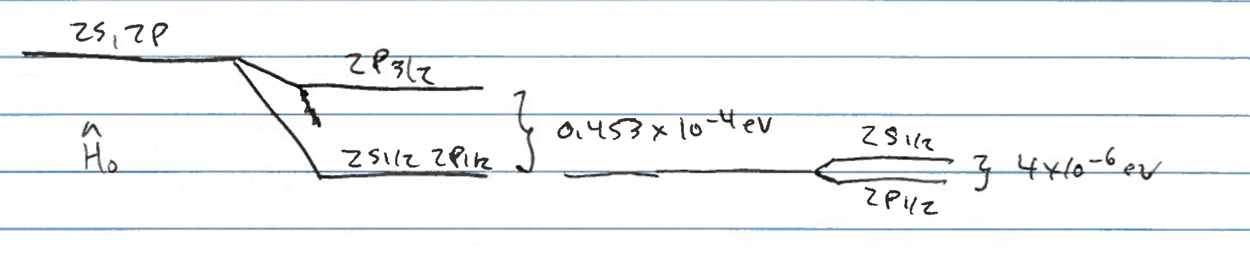
2.) The lowest excited states are \(2 P_{1 /
2} \text{ and } 2 S_{1 / 2}\) which are not split from each other
since the shift depends only on \(j\).
Experimentally they are split (called the Lamb shift), which can be
understood only with quantum electrodynamics (field theory);
3.) By choosing the \(jmls\) basis
we did not need to actually use degenerate perturbation theory because
we found the \(\parallel\)
subspace.
In the next lecture, we will need the degenerate formalism when we
examine the Zeeman effect.