Introduction to scattering

Start with time-dependent Schrodinger equation in coordinate basis \[i \hbar \frac{\partial}{\partial t} \psi(\mathbf{r}, t)=\left(-\frac{\hbar^{2}}{2 m} \nabla^{2}+V(\mathbf{r})\right) \psi(\mathbf{r}, t).\] The probability density to find the particle in the region around \(\mathbf{r}\) is \[\rho(\mathbf{r}, t)=|\psi(\mathbf{r}, t)|^{2}=\psi^{*}(\mathbf{r}, t) \psi(\mathbf{r}, t).\] The equation of continuity says that the change in the particle density must arise from the flow of currents, since particles are not created or destroyed. So \[\frac{d}{d t} \rho(\mathbf{r}, t)+\mathbf{\nabla} \cdot \mathbf{J}(\mathbf{r}, t)=0\] is the equation of continuity (recall electromagnetism).
We use this equation to find \(\mathbf{J}\): \[\frac{d}{d t} \rho(\mathbf{r}, t)=\frac{\partial}{\partial t} \psi^{*}(\mathbf{r}, t) \psi(r, t)+\psi^{*}(\mathbf{r}, t) \frac{\partial}{\partial t} \psi(\mathbf{r}, t).\] But \[\frac{\partial}{\partial t} \psi=\frac{i \hbar}{2 m} \nabla^{2} \psi+\frac{V}{i \hbar} \psi \qquad \text{and}\quad \frac{\partial}{\partial t} \psi^{*}=-\frac{i \hbar}{2 m} \nabla^{2} \psi^{*}+\frac{V}{i \hbar} \psi^{*}\] So \[\begin{aligned} \frac{d}{d t} \rho(\mathbf{r}, t) & =\frac{i \hbar}{2 m}\left(\psi^{*} \nabla^{2} \psi-\nabla^{2} \psi^{*} \psi\right)+\frac{V}{i \hbar}\left(\psi^{*} \psi-\psi^{*} \psi\right) \\ & =\mathbf{\nabla} \cdot \frac{i \hbar}{2m}\left(\psi^{*} \mathbf{\nabla} \psi-\mathbf{\nabla} \psi^{*} \psi\right) \quad \text { because } \mathbf{\nabla} \psi^{*} \cdot \mathbf{\nabla} \psi \text { terms cancel } \\ \Rightarrow& \boxed{\mathbf{J}= \frac{\hbar}{2 i m}\left(\psi^{*} \mathbf{\nabla} \psi-\mathbf{\nabla} \psi^{*} \psi\right)} \end{aligned}\]

Check: for a free particle \[\begin{aligned} \psi_{\text{free}}(\mathbf{r}, t)&=e^{i \mathbf{k} \cdot \mathbf{r}-i \frac{\hbar k^{2}}{2 m} t} \\ \mathbf{J}&=\frac{\hbar \mathbf{k}}{2 m} \times 2 \psi^{*} \psi=\frac{\hbar \mathbf{k}}{m} \psi^{*}(\mathbf{r}, t) \psi(\mathbf{r}, t) \end{aligned}\] But \(\frac{\hbar \mathbf{k}}{m}=\mathbf{v}= \text{ velocity}\) \(\Rightarrow\) current takes probability to find particle at position \(\mathbf{r}\) at time \(t\) and multiplies by the particle’s velocity. This is what a current should be.

Example: Scattering in one dimension

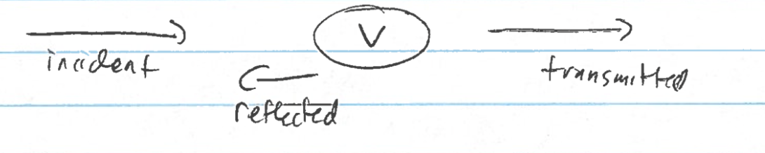
Simple example of 1D scattering—delta function potential at \(x=0\): \[V(x)=-\lambda \delta(x) \quad \lambda>0\] We have an incident wave from the left (looks like \(e^{ikx}\) far away)

So for \[\begin{aligned} x < 0 \qquad &\psi(x, t)=\psi_{\text {incident }}(x, t)+\psi_{\text {reflected }}(x, t)\\ x>0 \qquad &\psi(x, t)=\psi_{\text{transmitted}}(x,t) \quad \text{ assume stationary so no } t \text{ dependence} \end{aligned}\] \[\psi(x,t) =\left\{\begin{array}{cc} A(e^{ikx}+re^{-ikx}) & \quad x<0 \\ Ate^{ikx} & \quad x>0 \end{array} \right .\] \(r=\) Reflection amplitude \(\qquad t=\) Transmission amplitude
Now, we use the fact that \(\psi(x)\) is continuous across \(x=0\). This implies that \(A(1+r)=A t\) or \(1+r=t\).
Now, the potential vanishes everywhere except at \(x=0\). But, \(\left.\frac{d \psi}{d x}\right|_{x=0^{+}}-\left.\frac{d \psi}{d x}\right|_{x=0^{-}}=\int_{x=0^{-}}^{x=0^{+}} d x \frac{d^{2} \psi}{d x^{2}}=-\frac{2 m}{\hbar^{2}} \int_{x=0^{-}}^{x=0^{+}} d x\frac{-\hbar^{2}}{2 m} \frac{d^{2} \psi}{d x^{2}}\) and \(-\frac{\hbar^{2}}{2m} \frac{d^{2} \psi}{d x^{2}}=(E-V(x)) \psi\), so \[\left.\frac{d \psi}{d x}\right|_{x=0^{+}}-\left.\frac{d \psi}{d x}\right|_{x=0^{-}}=-\frac{2 m }{\hbar^{2}} E\left(\underbrace{\psi\left(x{=}0^{+}\right)-\psi\left(x{=}0^{-}\right)}_{0 \text{ since } \psi\text{ is continuous} }\right)-\frac{2 m \lambda}{\hbar^{2}} \psi(x{=}0)\] From this result, we can read off what the amplitudes are, so \[Aikt - Aik(1-r)=-\frac{2 m \lambda}{\hbar^{2}} A t \qquad \text { with } r=t-1.\] Hence, \[i k(t-1+t-1)=-\frac{2 m \lambda}{\hbar^{2}} t \qquad \text{and}\quad t=\frac{2 i k}{2 i k+\frac{2 m \lambda}{\hbar^{2}}}=\frac{+i \frac{\hbar^{2} k}{m \lambda}}{1+\frac{i \hbar^{2} k}{m \lambda}}.\] Simplifying, we have \[\boxed{ r=t-1=-\frac{1}{1+i \frac{\hbar^{2} k}{m \lambda}} \quad \text{and} \quad t=\frac{+i \frac{\hbar^2 k}{m \lambda}}{1+ i\frac{\hbar^{2} k}{m \lambda}} }\]

Note that these results satisfy \(|r|^{2}+|t|^{2}=1\) \[\begin{aligned} & |r|^{2}=R=\text { reflection coefficient } \\ & |t|^{2}=T=\text { transmission coefficient } \end{aligned}\] \(R+T=1\) is a consequence of conservation of probability, hence it always holds.

Formal theory for one-dimensional scattering

Now we treat a more formal theory of one -dimensional scattering.

We start from time dependent Schrodinger equation \[i \hbar \frac{\partial}{\partial t}|\psi(t)\rangle=\left(\hat{H}_{0}+\hat{V}\right)|\psi(t)\rangle \quad \text{and}\quad \hat{H}_{0}=\frac{\hat{P}^{2}}{2 m}=\text { kinetic energy. }\]

We define the Green’s function to satisfy \[\left(i \hbar \frac{\partial}{\partial t}-\hat{H}_{0}\right) \hat{G}_{0}\left(t, t^{\prime}\right)=\delta\left(t-t^{\prime}\right) \quad \text { which is called the equation of motion }\]

Since the delta function acts like a unit matrix, one can think of Green’s function as the inverse of the left most operator in the above equation (\(M^{-1}M=\mathbf{I}\)).
Since \(G_0\) has a delta function in its equation of motion, it must be discontinuous at \(t=t^{\prime}\).
Immediately, we break up the Green’s function into its two different pieces \[\begin{aligned} & \hat{G}_{0}\left(t, t^{\prime}\right)=\hat{G}_{0+}\left(t, t^{\prime}\right)+\hat{G}_{0-}\left(t, t^{\prime}\right) \\ & \hat{G}_{0 +}\left(t, t^{\prime}\right)=-\frac{i}{\hbar} \theta\left(t-t^{\prime}\right) e^{-i \hat{H}_{0}\left(t-t^{\prime}\right)/\hbar} \quad \text { retarded } \\ & \hat{G}_{0-}\left(t, t^{\prime}\right)=\frac{i}{\hbar}\theta\left(t^{\prime}-t\right) e^{-i \hat{H}_{0}\left(t-t^{\prime}\right) / \hbar} \quad\quad \text { advanced } \end{aligned}\] This solves the equation of motion, where \[\theta(t)=\left[\begin{array}{ll} 0 & t<0 \\ 1 & t>0 \end{array} \quad \text { and } \quad \frac{d}{d t} \theta(t)=\delta(t)\right.\] as can be seen by noting \(\frac{d}{d t} \theta(t)=0\) everywhere except at \(t=0\) where we have that \(\int_{t=0-}^{t=0+} \frac{d}{d t} \theta(t) d t =\theta\left(t{=}0{+}\right)-\theta(t{=}0-) =1-0=1\). So \(\frac{d}{d t} \theta(t)=0\) everywhere and \(\int_{0-}^{0+} d t \frac{d}{d t} \theta(t)=1 \Rightarrow\) delta function.
Using \(\hat{G}_{0}\) we find \[|\psi(t)\rangle=\left|\psi_{0}(t)\right\rangle+\int_{-\infty}^{+\infty} d t^{\prime} \hat{G}_{0}\left(t, t^{\prime}\right) \hat{V}\left(t^{\prime}\right)|\psi(t)\rangle\] Where \(\left|\psi_{0}(t)\right\rangle\) is the free quantum state, which satisfies \[\left.\left.i \hbar\frac{ d}{d t} \right\rvert\, \psi_{0}(t)\right\rangle=\hat{H}_{0}\left|\psi_{0}(t)\right\rangle.\]

Proof: \[\underbrace{\left(i \hbar \frac{d}{d t}-\hat{H}_{0}\right)}_{\text{from R.H.S}}|\psi(t)\rangle=\underbrace{\left(i \hbar \frac{d}{d t}-\hat{H}_{0}\right)}_{\text{is zero}}\left|\psi_{0}(t)\right\rangle+\underbrace{\hat{V}(t)|\psi(t)\rangle}_{\text{from full Schro. eq'n}}.\]

Now multiply by the inverse-operator from the left \[\begin{aligned} & \left(i\hbar\frac{d}{d t}-\hat{H}_{0}\right)^{-1} \text { on the left } \\ & |\psi(t)\rangle=\left|\psi_{0}(t)\right\rangle+\int d t^{\prime}\left(i \hbar \frac{d}{d t}-\hat{H}_{0}\right)^{-1}_{t,t^{\prime} \text{ matrix element}} \underbrace{\hat{V}(t^{\prime})\left|\psi\left(t^{\prime}\right)\right\rangle}_{\text{vector}} \\ \end{aligned}\] where the \(t,t'\) matrix element of the inverse operator is the Green’s function. Note that matrix multiplication of a continuous operator requires an integration over one index.
But \(\hat{G}_{0}(t, t^{\prime})\) is the inverse operator from the equation of motion, so

\[|\psi(t)\rangle=\left|\psi_{0}(t)\right\rangle+\int dt^{\prime} \hat{G}_{0}\left(t, t^{\prime}\right) \hat{V}\left(t^{\prime}\right)\left|\psi\left(t^{\prime}\right)\right\rangle\]

Now substitute in \(\hat{G}_{0}=\hat{G}_{0+}\) only because we are interested in retarded solutions which build up in time from the history of what happened for all earlier times. If you like, this is a postulate where we are introducing an "arrow of time".
So we get \[|\psi(t)\rangle=\left|\psi_{0}(t)\right\rangle-\frac{i}{\hbar} e^{-i \hat{H}_{0} t/\hbar} \int_{-\infty}^{t} d t^{\prime} e^{+i \hat{H}_{0} t^{\prime} / \hbar} \hat{V}\left(t^{\prime}\right)\left|\psi\left(t^{\prime}\right)\right\rangle\] as \(t \rightarrow-\infty \quad|\psi(t)\rangle \rightarrow\left|\psi_{0}(t)\right\rangle\) which is what we want if \(V\) is bounded.
Hence one can also view this choice as a way to satisfy the boundary condition.
Now, unlike bound state problems, when \(E>V\), we expect there to be a continuum of possible states. Let \(E\) be the energy of the initial state such that \[\begin{aligned} & \left|\psi_{0}(t)\right\rangle=e^{-i E t / \hbar}\left|\psi_{0}\right\rangle \quad \text { as } t \rightarrow-\infty \\ & |\psi(t)\rangle=e^{-i E t / \hbar}|\psi\rangle \text { as } t \rightarrow-\infty \end{aligned}\] Since we expect energy to be conserved if \(\hat{V}\) is independent of time, we expect the energy to stay at \(E\) for all time. Hence we write \[|\psi(t)\rangle=e^{-i E t / \hbar}|\psi\rangle \text { for all } t \text {. }\] Then we get \[|\psi\rangle=\left|\psi_{0}\right\rangle-\frac{i}{\hbar} e^{-i\left(\hat{H}_{0}-E\right) t / \hbar} \int_{-\infty}^{t} d t^{\prime} e^{i\left(H_{0}-E\right) t^{\prime}/\hbar} \hat{V}|\psi\rangle.\]

It is mathematically convenient to think of \(\hat{V}\) being turned on over some time interval in the infinite past, so we let \(\hat{V} \rightarrow \hat{V} e^{\delta t / \hbar} \qquad \delta \rightarrow 0^{+}\). This may sound like an odd thing to do, but it helps control some infinities one gets, if we do not do it.

Substituting in, we can now integrate \[\begin{aligned} |\psi\rangle & \left.=\mid \psi_{0}\right\rangle-\frac{i}{\hbar} e^{-i\left(\hat{H_{0}}-E\right) t/\hbar} \int_{-\infty}^{t} d t^{\prime} e^{i\left(\hat{H}_{0}-E\right) t^{\prime} / \hbar} e^{\delta t^{\prime} / \hbar} \hat{V}|\psi\rangle \\ & \left.=\mid \psi_{0}\right\rangle-\left.\frac{i}{\hbar} e^{-i\left(\hat{H}_{0}-E\right) t / \hbar} \frac{\hbar e^{i\left(\hat{H}_{0}-E\right) t^{\prime} / \hbar+\delta t^{\prime} / \hbar}}{i\left(\hat{H}_{0}-E\right)+\delta}\right|_{-\infty} ^{t} \hat{V} | \psi\rangle \end{aligned}\] The \(e^{\delta t^{\prime} / \hbar}\) makes the contribution vanish as \(t^{\prime} \rightarrow-\infty\) and we take the limit \(\delta \rightarrow 0^{+}\) for the \(e^{\delta t / \hbar}\) term so it approaches 1 and we obtain \[\begin{aligned} & |\psi\rangle=\left|\psi_{0}\right\rangle-\frac{e^{-i\left(\hat{H}_{0}-E ) t / \hbar\right.} e^{i\left(\hat{H}_{0}-E ) t\right.}}{\hat{H}_{0}-E-i \delta} \hat{V}|\psi\rangle \\ & |\psi\rangle=|\psi _0\rangle+\frac{i}{E-\hat{H}_{0}+i \delta} \hat{V}|\psi\rangle \end{aligned}\]

This is called the Lippman-Schwinger equation.