Last time, we derived the Lippman-Schwinger equation: \[|\psi\rangle = |\psi_0\rangle + \frac{1}{E - \hat{H}_0 + i\delta} \hat{V} |\psi\rangle.\] Let’s examine it in coordinate space by multiplying by \(\langle x|\) on the left and introducing the complete set of states \(\int |x'\rangle \langle x'| = \mathbb{I}\) between the fraction and the \(\hat{V}\): \[\psi(x) = \psi_0(x) + \int dx' \, \langle x| \frac{1}{E - \hat{H}_0 + i\delta} |x'\rangle V(x') \psi(x').\] Introduce the complete set of states \(\int |p\rangle \langle p| \, dp = \mathbb{I}\) on the left to get: \[\langle x| \frac{1}{E - \hat{H}_0 + i\delta} |x'\rangle = \int dp \, \langle x|p\rangle \langle p| \frac{1}{E - \hat{H}_0 + i\delta} |p\rangle \langle p|x'\rangle.\] But \(\langle x|p\rangle = \frac{e^{ipx/\hbar}}{\sqrt{2\pi \hbar}}\) and \(\hat{H}_0 |p\rangle = \frac{p^2}{2m} |p\rangle\), where \(\frac{p^2}{2m}\) is a number. Thus: \[\begin{aligned} \langle x| \frac{1}{E - \hat{H}_0 + i\delta} |x'\rangle &= \int dp \, \frac{e^{ipx/\hbar}}{\sqrt{2\pi \hbar}} \frac{1}{E - \frac{p^2}{2m} + i\delta} \frac{e^{-ipx'/\hbar}}{\sqrt{2\pi \hbar}}\\ &= \int dp \, \frac{e^{i p(x - x')/\hbar}}{2\pi \hbar} \frac{1}{\left (\sqrt{E + i\delta} - \frac{p^2}{2m}\right )\left ( \sqrt{E + i\delta} + \frac{p^2}{2m}\right )} \end{aligned}\] You can integrate this using residues. If you don’t know how to do this, don’t worry. The answer is: \[\begin{aligned} \langle x| \frac{1}{E - \hat{H}_0 + i\delta} |x'\rangle &= -i \sqrt{\frac{2m}{\hbar^2}} \frac{1}{2\sqrt{E}} \left[ \Theta(x - x') e^{i\sqrt{\frac{2mE}{\hbar^2}} (x - x')} + \Theta(x' - x) e^{-i\sqrt{\frac{2mE}{\hbar^2}} (x - x')} \right] \\ &= -i \frac{\sqrt{2mE}}{\hbar}\frac{1}{2E}\left[ \Theta(x - x') e^{i{\sqrt{2mE}} (x - x')/\hbar} + \Theta(x' - x) e^{-i{\sqrt{2mE}} (x - x')/\hbar} \right] \end{aligned}\] Let: \(k = \sqrt{\frac{2mE}{\hbar^2}}\) and choose \(\psi_0(x) = e^{ikx}\), corresponding to an incident wave moving to the right. Then: \[\begin{aligned} \psi(x) &= e^{ikx} - \frac{ik}{2E} \int_{-\infty}^x e^{-ik(x - x')} V(x') \psi(x') \, dx' - \frac{ik}{2E} \int_x^{\infty} e^{ik(x - x')} V(x') \psi(x') \, dx' \\ &=e^{ikx} \left( 1 - \frac{ik}{2E} \int_{-\infty}^x e^{-ik(x - x')} V(x') \psi(x') \, dx' \right) - \frac{ik}{2E} e^{-ikx} \int_x^{\infty} e^{ikx'} V(x') \psi(x') \, dx'. \end{aligned}\] If we consider the limit when \(x \to +\infty\): \[t = 1 - \frac{ik}{2E} \int_{-\infty}^\infty e^{-ikx'} V(x') \psi(x') \, dx'\] and in the limit when \(x \to -\infty\): \[r = -\frac{ik}{2E} \int_{-\infty}^\infty e^{ikx'} V(x') \psi(x') \, dx'.\] Since \(\psi(x)\) represents scattering to the right, we write \(|\psi\rangle = |\psi_\rightarrow\rangle\) and so: \[\psi_0(x) = e^{ikx} = \langle x|\psi_{0\rightarrow}\rangle\quad\text{and}\quad e^{-ikx} = \langle x|\psi_{0\leftarrow}\rangle\] Thus, we can write: \[r_{\rightarrow} = -\frac{ik}{2E} \langle \psi_{0\leftarrow} | \hat{V} | \psi_{\rightarrow} \rangle \quad\text{and}\quad t_\rightarrow = 1 - \frac{ik}{2E} \langle \psi_{0\rightarrow} | \hat{V} | \psi_\rightarrow \rangle.\]
Let: \[|\psi\rangle = |\psi_0\rangle + \frac{1}{E - \hat{H}_0 + i\delta} \hat{V} |\psi\rangle\] and define \[\frac{1}{E - \hat{H}_0 + i\delta} = \hat{G}_{0+}(E)\] so: \[|\psi\rangle = \left[ 1 - \hat{G}_{0+}(E)\hat{V} \right]^{-1} |\psi_0\rangle.\] You may want to compare this with how we had organized pertrubation theory for bound states previously. The reflection \(r_\rightarrow\) and transmission \(t_\rightarrow\) coefficients are given by: \[\begin{cases} r_\rightarrow = -\frac{ik}{2E} \langle \psi_0 | \hat{V} \left[ 1 - \hat{G}_{0+}(E) \hat{V} \right]^{-1} |\psi_0\rangle \\ t_\rightarrow = 1 - \frac{ik}{2E} \langle \psi_0 | \hat{V} \left[ 1 - \hat{G}_{0+}(E) \hat{V} \right]^{-1} |\psi_0\rangle. \end{cases}\] Expand in a geometric series: \[|\psi_\rightarrow\rangle = \sum_{n=0}^\infty \left( \hat{G}_{0+}(E) \hat{V} \right)^n |\psi_{0\rightarrow}\rangle,\] giving us: \[\begin{cases} r_\rightarrow = -\frac{ik}{2E} \sum_{n=0}^\infty \langle\psi_{0\leftarrow} | \hat{V} \left( \hat{G}_{0+}(E) \hat{V} \right)^n |\psi_{0\rightarrow}\rangle \\ t_\rightarrow = 1 - \frac{ik}{2E} \sum_{n=0}^\infty \langle \psi_{0\rightarrow} | \hat{V} \left( \hat{G}_{0+}(E) \hat{V} \right)^n |\psi_{0\rightarrow}\rangle. \end{cases}\] This is a formal series, similar to perturbation theory for bound states, that we can expand to obtain subsequently more accurate approximations to the scattering problem solutions. The case when \(n=1\) is called the Born Approximation: \[\begin{cases} |\psi^{\text{Born}}_\rightarrow\rangle = |\psi_{0\rightarrow}\rangle + \hat{G}_{0+}(E) \hat{V} |\psi_{0\rightarrow}\rangle \\ \psi^{\text{Born}}_\rightarrow(x) = e^{ikx} + \int_{-\infty}^\infty dx' \, \hat{G}_{0+}(x - x') V(x') e^{ikx'}\\ r^{\text{Born}}_\rightarrow = -\frac{ik}{2E} \langle \psi_{0\leftarrow} | \hat{V} |\psi_{0\rightarrow}\rangle = -\frac{ik}{2E} \int_{-\infty}^\infty dx \, V(x) e^{2ikx} \\ t^{\text{Born}} _\rightarrow= 1 - \frac{ik}{2E} \langle\psi_{0\rightarrow} | \hat{V} |\psi_{0\rightarrow}\rangle = 1 - \frac{ik}{2E} \int_{-\infty}^\infty dx \, e^{ikx} V(x) e^{ikx} \approx e^{\frac{ik}{2E} \int_{-\infty}^\infty dx \, V(x)} \end{cases}\] Since we assume \(\hat{V}\) is small, \(r^{\text{Born}}_\rightarrow \sim 0\) and \(t^{\text{Born}}_\rightarrow \sim 1\). Hence, the Born approximation works well when most of the wave is transmitted.
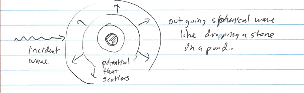
Recall expansion of plane wave in spherical harmonics with \(E= \frac{\hbar^2k^2}{2m}\) and thus \(k = \frac{\sqrt{2mE}}{\hbar}\): \[e^{i kr\cos\theta} = \sum_{\ell=0}^\infty (2\ell + 1) i^\ell j_\ell(kr) P_\ell(\cos\theta),\] where \(j_\ell(kr) = \sqrt{\frac{\pi}{2kr}} J_{\ell+\frac{1}{2}}(kr)\) is a spherical Bessel function and \(P_\ell(\cos\theta)\) a Legendre polynomial. Recall as well that as \(r \to \infty\), we have: \[j_\ell(kr) \to \frac{1}{kr} \sin\left(kr - \frac{\ell\pi}{2}\right).\] Thus for \(r \to \infty\): \[f_\ell(r) \to C_\ell \sin\left(kr - \frac{\ell\pi}{2}\right)= C_\ell \left(e^{i(kr - \frac{\ell\pi}{2})} - e^{-i(kr - \frac{\ell\pi}{2})}\right),\] where the term \(e^{i(kr - \frac{\ell\pi}{2})}\) is an outgoing wave and \(e^{-i(kr - \frac{\ell\pi}{2})}\) an incoming wave.
For an interacting case, where \(V(r) \to 0\) faster than the centrifugal potential \(\frac{\hbar^2 \ell(\ell+1)}{2mr^2}\), we expect as \(r\to\infty\) \[f_\ell(r) \to A_\ell(k) \left(e^{-ikr} + r_\ell(k) e^{ikr}\right)\] where \(A_\ell(k)\) is a constant, \(e^{-ikr}\) an incident wave, and \(r_\ell(k) e^{ikr}\) a reflected wave. This is because nothing can transmit through \(r=0\) (recall analogy to a 1D infinite wall at \(r=0\)). But in 1D we have \(R+T=1\) which implies if \(T=0\), then \(R=1\). Thus \(r = e^{i\phi}=\) phase and we write: \[r_\ell(k) = -e^{i(2\delta_\ell(k) - \ell\pi)}\] with \(\delta_\ell(k)\) being the \(\ell\)-th partial wave phase shift. Substituting in to find: \[\begin{aligned} f_\ell(r) &\to A_\ell(k) \left(e^{-ikr} - e^{i(2\delta_\ell(k) - \ell\pi + kr)}\right)\\ &= A_\ell(k) e^{i(\delta_\ell(k) - \frac{\ell\pi}{2})} 2i \sin\left(kr + \delta_\ell(k) - \frac{\ell\pi}{2}\right)\\ &= B_\ell(k) \sin\left(kr + \delta_\ell(k) - \frac{\ell\pi}{2}\right). \end{aligned}\] For the free case, \(V=0\) and \(\delta_\ell(k) = 0\) for all \(\ell\) and \(k\).
Example 1. Consider a spherical well as pictured below.
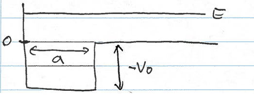
Define: \[\begin{cases} k_1 = \frac{1}{\hbar} \sqrt{2m(E + V_0)} \quad \text{for } r < a,\\ k_2 = \frac{1}{\hbar} \sqrt{2mE} \quad \text{for } r > a, \end{cases}\] with \(E>0\). Then we have: \[R_\ell(r) = \begin{cases} A_\ell(E) j_\ell(k_1 r), & r < a, \\ B_\ell(E) j_\ell(k_2 r) + C_\ell(E) \eta_\ell(k_2 r), & r > a, \end{cases}\] where there is no restriction on the wave functions for \(r > a\) since \(r = 0\) is not within this region. Now, continuity of \(\psi\) at \(r = a\) tells us: \[A_\ell(E) j_\ell(k_1 a) = B_\ell(E) j_\ell(k_2 a) + C_\ell(E) \eta_\ell(k_2 a).\] And continuity of \(\frac{d\psi}{dr} = \psi'\) at \(r = a\) tells us: \[k_1 A_\ell(E) j_\ell'(k_1 a) = k_2 B_\ell(E) j_\ell'(k_2 a) + k_2 C_\ell(E) \eta_\ell'(k_2 a).\] We now want to solve for the coefficients \(B_\ell(E)/ A_\ell(E)\) and \(C_\ell(E)/A_\ell(E)\). We find:\[\frac{B_\ell(E)}{A_\ell(E)} = \frac{k_2 \eta_\ell(k_2 a) j_\ell'(k_1 a) - k_1 j_\ell(k_1 a) \eta_\ell'(k_2 a)}{k_2 \eta_\ell(k_2 a) j_\ell'(k_2 a) - k_2 j_\ell(k_2 a) \eta_\ell'(k_2 a)},\] and: \[\frac{C_\ell(E)}{A_\ell(E)} = \frac{k_2 j_\ell'(k_2 a) j_\ell(k_1 a) - k_1 j_\ell'(k_1 a) j_\ell(k_2 a)}{k_2 \eta_\ell(k_2 a) j_\ell'(k_2 a) - k_2 j_\ell(k_2 a) \eta_\ell'(k_2 a)}.\] Note that: \[\eta_\ell(p) \to -\frac{1}{p} \cos\left(p - \ell \frac{\pi}{2}\right).\] Yes, it is a mess. One would want to ultimately extract the scattering phase shifts from this, but we are not going to show that here.