In this lecture, we will discuss how to measure the quadratures \(\hat{Q}_{l}\) and \(\hat{P}_{l}\), how to reduce the uncertainty in one value at the expense of the other and how LIGO employs these ideas for higher precision and to see farther out into the universe.
To start, we note that one cannot directly measure an oscillating electric field of visible light because it oscillates too fast. The fastest oscilloscopes work at about 100 GHz , while light’s oscillation frequency at \(10^{14}-10^{15} \mathrm{~Hz}\) is \(3-4\) orders at magnitude faster. Nevertheless, there are schemes that do allow us to measure the fields of light by employing clever techniques. The first we will discuss is heterodyne detection. This involves measuring signals from two light beams, whose frequency differs by a small amount, and observing the beats of those signals, which oscillate much more slowly. Let’s see how this works.

Heterodyne detection

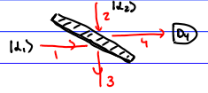
In this experiment, we send in the weak light \(\left|\alpha_{1}\right\rangle\) that we want to measure and the strong light \(\left| \alpha_{2}\right\rangle\), used to "boost" the signal. We measure the photocurrent in channel 4 .

\[\begin{aligned} & \left.\mid \psi_{\text{in}}\right\rangle=\left|\alpha_{1}\right\rangle \otimes\left|\alpha_{2}\right\rangle \\ & i_{4}=q_{e} S w^{(1)}\left(r_{4}, t\right)=q_{e} S s\left\|E_{4}^{(+)}\left\langle r_{4}, t \mid \psi_{\text{in}}\right\rangle\right\|^{2} \\ & E_{4}^{(+)}=t E_{1}^{(+)}-r E_{2}^{(+1)}. \end{aligned}\] Here, \(S\) is the cross-sectional area and \(r\) and \(t\) are the reflection and transmission amplitudes. Assume the frequencies \(w_{1}\) and \(w_{2}\) of the light input to those respective channels are close, so that we can approximate \[\begin{aligned} & \mathcal{E}_{omega_{1}}^{(1)} \sim \mathcal{E}_{\omega_{2}}^{(1)} \sim \mathcal{E}_{\omega}^{(1)} \quad \omega=\frac{\omega_{1} +\omega_{2}}{2} \\ i_{4}&=q_{e} S s\left(\mathcal{E}_{\omega}^{(1)}\right)^{2}\left\|\left(t \alpha_{1} e^{-i \omega_{1} t}-r \alpha_{2} e^{-i \omega_{2} t}\right)\left|\psi_{i}\right\rangle\right\|^{2} \\ & =q_{e} S_{s}\left(\mathcal{E}_{\omega}^{(1)}\right)^{2}\left\{|t|^{2}\left.|\left.\alpha_{1}\right|^{2}+|r|^2 |{\alpha_{2}}|^{2}-2 \operatorname{Re}\left(r t^{*} e^{i\left(\omega_{1}-\omega_{2}\right) t} \alpha_{1}^{*} \alpha_{2}\right)\right\}\right. \end{aligned}\] Let \(\alpha_{1}=\left|\alpha_{1}\right| e^{i \phi_{1}}\), \(\alpha_{2}=|\alpha_{2}| e^{i \phi_{2}}\), and assume \(r\) and \(t\) are real, then \[\left.i_{4}=q_{e} Ss\left(\mathcal{E}_{\omega}^{(1)}\right)^{2} \ \left\{|t|^{2}\left|\alpha_{1}\right|^{2}+|r|^{2}\left|\alpha_{2}\right|^{2}-2 r t\left|\alpha_{1}\right|\left|\alpha_{2}\right| \cos \left[\left( \omega_{1}-\omega_{2}\right) t-\phi_{1}+\phi_{2}\right.\right]\right\}\]

Recall \(s(\mathcal{E}^{(1)}_\omega)^2 = \frac{\eta}{ST}\) for light moving in a cylindrical quantization volume. Recall as well that \(|\alpha|^{2}\) is proportional to the number of photons in the quantization volume since \(\langle\alpha| \hat{N}|\alpha\rangle=|\alpha|^{2}\).

This number of photons increases as the length \(L=cT\) increases by considering longer time intervals for the measurement. But \(\Phi_{\text {phot }}{=}\text{photon flux} = \frac{|\alpha|^2}{T}\) is independent of \(T\) (you can think of this as the "density" of photons). The beam intensity, or energy density, is \(\Phi=\Phi_{\text {phot }} \cdot \hbar \omega_{l}\) so the beam intensity satisfies \(\frac{\Phi}{\hbar \omega_{l}}=\frac{\left|\alpha_{l}\right|^{2}}{T}\) or \[\left|\alpha_{l}\right|=\sqrt{\frac{\Phi T}{\hbar \omega_{l}}}.\] So the heterodyne signal becomes \[i_{4}(t)=\eta q_{e}\left\{t^{2} \Phi_{1}^{\text{phot}}+r^{2} \Phi_{2}^{\text{phot}}-2 r t \sqrt{\Phi_{1}^{\text{phot}} \Phi_{2}^{\text{phot}}} \cos \left[\left(\omega_{1}-\omega_{2}) t-\phi_{1}+\phi_{2}\right]\right.\right\}.\]

If we tune \(r\) and \(t\) such that \(t^{2} \Phi_{1}^{\text {phot}}=r^{2} \Phi_{2}^{\text {phot}}\), then \(i_{4}(t)=2 t^{2} \Phi_{1}^{\text {phot}} \eta q_{e}\left(1-\cos \left(\left(\omega_{1}-\omega_{2}\right) t-\phi_{1}+\phi_{2}\right)\right)\), which says the visibility is equal to \(1\).

The idea is that instead of measuring the small amplitude \(\Phi_{1}^{\text {phot}}\), we measure a much larger amplitude \(\sqrt{\Phi_{1}^{\text {phot}} \Phi_{2}^{\text {phot}}}\). But one must examine the signal to noise ratio to see if there is a true gain: \[i_{\text{direct}} = \eta q_e \Phi_1^{\text{phot}} \qquad i_{\text{hetero}} = \eta q_e r t \sqrt{\Phi_{1}^{\text {phot}} \Phi_{2}^{\text {phot}}}.\]

The noise is white noise (also called shot noise). I don’t have time to derive this here, but it is given by \(\Delta i_{\text {direct }}=\sqrt{2 q_{e} i_{\text {direct}} \Delta f}\) with \(\Delta f=\frac{1}{T}={\text {bandwidth }}\). So \[\begin{aligned} \left(\frac{\text{Signal}}{\text{Noise}}\right)_\text{direct} & = \frac{i_{\text{direct}}}{\sqrt{2q_ei_{\text{direct}} \Delta f}} = \sqrt{\frac{i_{\text{direct}}}{2q_e \Delta f}} = \sqrt{\frac{\eta \Phi_1^{\text{phot}}}{2 \Delta f}}\\ \left(\frac{\text{Signal}}{\text{Noise}}\right)_\text{hetero} & = \frac{\eta q_e r t \sqrt{\Phi_{1}^{\text {phot}} \Phi_{2}^{\text {phot}}}}{r\sqrt{2\underbrace{q_e^2}_{i\alpha q_e} \eta \underbrace{\Phi_2^{\text{Phot}}}_{\text{dominates the noise}} \Delta f}} = t\sqrt{\frac{\eta \Phi_1 ^{\text{Phot}}}{2 \Delta f}}\\ \end{aligned}\]

So there seems to be no gain. But this analysis ignored the dark current noise. This is a constant and can make it impossible to observe \(i_{\text{direct}}\) because it is so small. So with dark current, one can measure signals via heterodyning that are much smaller than the dark current if \(|\alpha_{2}|\) is large. We don’t have a gain in accuracy, but we lift the signal above the noise floor.

Balanced homodyne detection

This is very similar to heterodyning except now we take \(\omega_{1}=\omega_{2}, \mathbf{k}_{1}=\mathbf{k}_{2}, \boldsymbol{\mathcal{E}}_{1}=\boldsymbol{\mathcal{E}}_{2}\), so there is no oscillation. We measure now the difference in photocurrents \(i_{3}-i_{4}\). Note that this is the difference of two photocurrents, measured over a long time interval, not the coincidences.

Recall that

\[\begin{aligned} S T W_{3,4}^{(1)}(r, t) & =\eta\left.|\langle\psi| \hat{N}_{3,4}\right.| \psi\rangle|^{2} \\ i_{3,4} & =\eta \frac{q_{e}}{T}\left|\langle\psi| \hat{N}_{3,4}\right| \psi\rangle|^{2}. \end{aligned}\] We need to express \(\hat{N}_{3}-\hat{N}_{4}\) in terms of the input creation/annihilation operators. In balanced homodyne detection, we take \(r=t=\frac{1}{\sqrt{2}}\), so \[\begin{aligned} \hat{N}_{3} & =\left(r \hat{a}_{1}^{\dagger}+t \hat{a}_{2}^{\dagger}\right)\left(r \hat{a}_{1}+t \hat{a}_{2}\right) \\ & =\frac{1}{2}\left(\hat{a}_{1}^{\dagger} \hat{a}_{1}+\hat{a}_{2}^{\dagger}\hat{a}_{2}+\hat{a}_{1}^{\dagger}\hat{a}_{2}+\hat{a}_{2}^{\dagger}\hat{a}_{1}\right) \\ \hat{N}_{4} & =\left(t\hat{a}_{1}^{\dagger}-r \hat{a}_{2}^{\dagger}\right)\left(t \hat{a}_{1}-r \hat{a}_{2}\right) \\ & =\frac{1}{2}\left(\hat{a}_{1}^{\dagger}\hat{a}_{1}+\hat{a}_{2}^{\dagger} \hat{a}_{2}-\hat{a}_{1}^{\dagger} \hat{a}_{2}-\hat{a}_{2}^{\dagger}\hat{a}_{1}\right). \end{aligned}\] So, \(\hat{N}_{3}-\hat{N}_{4}=\hat{a}_{1}^{\dagger}\hat{a}_{2}+\hat{a}_{2}^{\dagger} \hat{a}_{1}\). We let \(\alpha_{2}=\alpha_{\text{LO} }=\left|\alpha_{\text{LO}}\right| e^{i \phi_{\text{LO}}}\) with \(\text{LO}= \text{local oscillator}\), then \[\begin{aligned} i_{3}-i_{4}= & \eta \frac{q_{e}}{T}\left\langle\psi_{1}\right| \hat{a}_{1}^{\dagger}\left|\psi_{1}\right\rangle\left|\alpha_{\text{LO}}\right| e^{i \phi_{\text{LO}}}+\left\langle\psi_{1}\right| \hat{a}_{1}\left|\psi_{1}\right\rangle |\alpha_{\text{LO}}| e^{-i \phi_{\text{LO}}} \\ = & \eta \frac{q_{e}}{T}\left|\alpha_{\text{LO}}\right|\left\langle\psi_{1}\right| \hat{a}_{1}^{\dagger} e^{i \phi_{\text{LO}}}+\hat{a}_{1} e^{-i \phi_{\text{LO}}}\left|\psi_{1}\right\rangle \\ = & \eta \frac{q_{e}}{T}\left|\alpha_{\text{LO}}\right|\{ \left\langle\psi_{1}\right| \hat{a}_{1}^{\dagger}+\hat{a}_{1}\left|\psi_{1}\right\rangle \cos \phi_{\text{LO}} \\ &\left.+i\left\langle\psi_{1}\right| \hat{a}_{1}^{\dagger} - \hat{a}_{1}\left|\psi_{1}\right\rangle \sin \phi_{\text{LO}}\right\} \end{aligned}\] Recall \(\hat{a}_{1}^{\dagger}+\hat{a}_{1} \propto \hat{Q}_{1}\) and \(i\left(\hat{a}_{1}^{\dagger}-\hat{a}_{1}\right) \propto \hat{P}_{1}\)
So using balanced homodyne detection, we can measure the quadrature operators as functions of the local oscillator phase. Note as well that the result is independent of the time interval \(T\) because the number of photons grows linearly in the time interval.

We need to now discuss fluctuations/noise.
\[\begin{aligned} \left(\hat{N}_{3}-\hat{N}_{4}\right)^{2}=\left(\hat{a}_{1}^{\dagger}\hat{a}_{2}+\hat{a}_{2}^{\dagger}\hat{a}_{1}\right)^{2}= & \hat{a}_{1}^{\dagger} \hat{a}_{1}^{\dagger} \hat{a}_{2} \hat{a}_{2}+\hat{a}_{1}^{\dagger} \hat{a}_{2} \hat{a}_{2}^{\dagger}\hat{a}_{1} \\ & +\hat{a}_{2}^{\dagger} \hat{a}_{1} \hat{a}_{1}^{\dagger} \hat{a}_{2}+\hat{a}_{2}^{\dagger} \hat{a}_{2}^{\dagger}\hat{a}_{1} \hat{a}_{1}. \end{aligned}\] Put into normal ordered form (all \(\dagger\)’s to the left) to find \[\begin{aligned} = & \hat{a}_{1}^{\dagger} \hat{a}_{1}^{\dagger} \hat{a}_{2} \hat{a}_{2}+\hat{a}_{2}^{\dagger} \hat{a}_{2}^{\dagger} \hat{a}_{1} \hat{a}_{1}+\hat{a}_{1}^{\dagger} \hat{a}_{2}^{\dagger} \hat{a}_{1} \hat{a}_{2}+\hat{a}_{1}^{\dagger} \hat{a}_{1} \\ & +\hat{a}_{2}^{\dagger} \hat{a}_{1}^{\dagger} \hat{a}_{1} \hat{a}_{2}+\hat{a}_{2}^{\dagger} \hat{a}_{2}+\hat{a}_{2}^{\dagger} \hat{a}_{2}^{\dagger} \hat{a}_{1} \hat{a}_{1} \end{aligned}\] When taking the average with respect to \(|\alpha_{\text{LO}}\rangle \qquad \hat{a}_2 \rightarrow \alpha_{\text{LO}} \quad \hat{\alpha}_2^{\dagger} \rightarrow \alpha_{\text{LO}}^*\) \[\begin{gathered} \left\langle\psi_{\text {in }}\right|\left(\hat{N}_{3}-\left.\hat{N}_{4}\right)^{2} | \psi_{\text {in }}\right.\rangle=\left|\alpha_{\text{LO}}\right|^{2}\left\{\left\langle\psi_{1}\right| \hat{a}_{1}^{\dagger} \hat{a}_{1}^{\dagger} | \psi_{1}\right.\rangle e^{+2 i \phi_{\text{LO}}}+\left\langle\psi_{1}\right| \hat{a}_{1} \hat{a}_{1} \mid \psi_{1}\rangle e^{-2 i \phi_{\text{LO}}} \\ \left.+\left\langle\psi_{1}\right| \hat{a}_{1}^{\dagger} \hat{a}_{1}\left|\psi_{1}\right\rangle+\left\langle\psi_{1}\right| \hat{a}_{1} \hat{a}_{1}^{\dagger}\left|\psi_{1}\right\rangle\right\}+\underbrace{\left\langle\psi_{1}\right| \hat{a}_{1}^{\dagger} \hat{a}_{1}\left|\psi_{1}\right\rangle}_{\text{neglect bc small compared to } |\alpha_{\text{LO}}|^2} \end{gathered}\] \[\begin{aligned} \Rightarrow\left(\Delta\left(N_{3}-N_{4}\right)\right)^2{\left.\mid \psi_{i n}\right\rangle}= & \left|\alpha_{\text{LO}}\right|^{2}\left\{\left\langle\psi_{1}\right|\left(\hat{a}_{1}^{\dagger} e^{i \phi_{\text{LO}}}+\hat{a}_{1} e^{-i \phi_{\text{LO}}}\right)^{2}\left|\psi_{1}\right\rangle\right. \\ & \left.-\left(\left\langle\psi_{1}\right.|\left(\hat{a}_{1}^{\dagger} e^{i \phi_{\text{LO}}}+\hat{a}_{1} e^{-i \phi_{\text{LO}}}\right)\left.|\psi_{1}\right\rangle\right)^{2}\right\} \\ = & \left|\alpha_{\text{LO}}\right|^{2}\left(\Delta\left(\hat{a}_{1}^{\dagger} e^{i \phi_{\text{LO}}}+\hat{a}_{1} e^{-i \phi_{\text{LO}}}\right)\right){\left|\psi_{1}\right\rangle}^{2}. \end{aligned}\]

As mentioned before, this is related to the quadrature operators. We can define \(\hat{Q}_{1}\left(\phi_{\text{LO}}\right)=\sqrt{\frac{\bar{\hbar}}{2}}\left(\hat{a}_{1}^{\dagger} e^{i \phi_{\text{LO}}}+\hat{a}_{1} e^{-i \phi_{\text{LO}}}\right)\) recalling \(\hat{Q}_{1}=\sqrt{\frac{\hbar}{2}}\left(\hat{a}_{1}+\hat{a}_{1}^{\dagger}\right) \quad \hat{P}_{1}=-i \sqrt{\frac{\hbar}{2}}\left(\hat{a}_{1}-\hat{a}_{1}^{\dagger}\right)\) says when \(\phi_{\text{LO}}=0\), we get \(Q\), when \(\phi_{\text{LO}}=\frac{\pi}{2}\) we get \(P\).

Note these are related to the dielectric field amplitude since \[\hat{E}(\mathbf{r}, t)=\sum_{l} \mathbf{\varepsilon}_{l} \mathcal{E}_{l}^{(1)} \sqrt{\frac{2}{\hbar}}\left\{-\hat{Q}_{l} \sin \left(\mathbf{k}_{l} \mathbf{r}-\omega_{l} t\right)-\hat{P}_{l} \cos \left(\mathbf{k}_{l} \cdot \mathbf{r}-\omega_{l} t\right)\right\}\] \(Q\) is the real part of the amplitude and \(P\) is imaginary part.
In general, we can consider \(\hat{Q}(\theta)\) and \(\hat{Q}\left(\theta+\frac{\pi}{2}\right)=\hat{P}(\theta)\). One can immediately verify that \([\hat{Q}(\theta), \hat{P}(\theta)]=i \hbar\).
We will use these to measure the field. \(\left.\quad\left|\psi_{1}\rangle=\right| \alpha_{1}\right\rangle \quad \alpha_{1}=\left|\alpha_{1}\right| e^{i \phi_{1}}\) \[\begin{aligned} \left\langle\psi_{1}\right| \hat{Q}(\theta)\left|\psi_{1}\right\rangle & =\sqrt{\frac{\pi}{2}}\left\langle\alpha_{1}\right| \hat{a}_{1}^{\dagger} e^{i \theta}+\hat{a}_{1} e^{-i \theta}\left|\alpha_{1}\right\rangle \\ & =\sqrt{2 \hbar} \cos \left(\theta-\phi_{1}\right)\left|\alpha_{1}\right| \\ \left\langle\psi_{1}\right| \hat{P}(\theta)\left|\psi_{1}\right\rangle & =-i \sqrt{\frac{\hbar}{2}}\left\langle\alpha_{1}\right|-\hat{a}_{1}^{\dagger} e^{i \theta}+\hat{a}_{1} e^{-i \theta}\left|\alpha_{1}\right\rangle \\ & =-\sqrt{2 \hbar} \sin \left(\theta-\phi_{1}\right)\left|\alpha_{1}\right|. \end{aligned}\]

Variances: \[\begin{aligned} \left\langle\psi_{1}\right| \hat{Q}(\theta)^{2}\left|\psi_{1}\right\rangle & =\frac{\hbar}{2}\left\langle\alpha_{1}\right| \hat{a}_{1}^{\dagger} \hat{a}_{1}^{\dagger} e^{2 i \theta}+\hat{a}_{1}^{\dagger} \hat{a}_{1}+\hat{a}_{1} \hat{a}_{1}^{\dagger}+\hat{a}_1{\hat{a}_{1}} \hat{e}^{-2 i \theta}\left|\alpha_{1}\right\rangle\\ & =\hbar\left|\alpha_{1}\right|^{2}\left(\cos 2\left(\theta-\phi_{1}\right)+1\right)+\frac{\hbar}{2} \\ & =2 \hbar|\alpha_1|^{2} \cos ^{2}\left(\theta-\phi_{1}\right)+\frac{\hbar}{2} \\ \left.\left\langle\psi_{1}\right| \hat{P}(\theta)^{2} \mid \psi_{1}\right.\rangle & \left.=-\frac{\hbar}{2}\left\langle\alpha_{1}\right| \hat{a}_{1}^{\dagger} \hat{a}_{1}^{\dagger} e^{2 i \theta}-\hat{a}_{1}^{\dagger} \hat{a}_{1}-\hat{a}_{1} \hat{a}_{1}^{\dagger}+\hat{a}_{1} \hat{a}_{1} e^{-2 i \theta}|\alpha_1|\right. \\ & =-\hbar\left|\alpha_{1}\right|^{2}\left(\cos 2\left(\theta-\phi_{1}\right)-1\right)+\frac{\hbar}{2} \\ & =2 \hbar\left|\alpha_{1}\right|^{2} \sin ^{2}\left.(\theta-\phi_{1} \left.)+\frac{\hbar}{2}\right.\right. .\\ \text { So }(\Delta Q(\theta))_{\psi_{1}} & =\sqrt{\frac{\hbar}{2}} = (\Delta P(\Theta))_{\psi_1}\\ (\Delta Q(\theta))_{\psi_{1}}(\Delta P(\Theta))_{\psi_1}& = \frac{\hbar}{2} = \text{ minimal uncertainty state} \end{aligned}\]

We can plot the uncertainty in a "phase space" \[{\text {Prob}}\left( Q_{1}, P_1\right)=\frac{1}{2 \pi \Delta Q_{1}^{2}} e^{-\frac{\left(Q_{1}-\langle \hat{Q}_{1}\rangle \right)^{2} + (P -\langle \hat{P}_l \rangle)^2}{2 \Delta Q_{1}^{2}}}\]

Use reduced variables \(\frac{Q}{\sqrt{2 \pi}}, \frac{P}{\sqrt{2 \pi}} \quad \frac{2 \Delta Q_{1}}{\sqrt{2 \pi}}=1\)

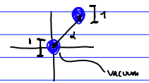
Time evolution, given by \(\alpha \rightarrow \alpha e^{i \omega t}\), is a clockwise rotation in a circle. The uncertainty, being a circle, is always the same for \(Q\) and \(P\).
Squeezed light trades off the uncertainty for \(Q\) to uncertainty in \(P\) or vice versa. Recall the Bogoliubov transformation form HW: \[\begin{aligned} & \hat{A}_{R}=\cosh R \hat{a}+\sinh R a^{\dagger} \quad \text{and}\quad\hat{A}_{R}^{\dagger}=\cosh R \hat{a}^{\dagger}+\sinh R \hat{a} \\ & {\left[\hat{A}_{R}, \hat{A}_{R}{ }^{\dagger}\right]=\left(\cosh ^{2} R-\sinh ^{2} R\right)=1}. \end{aligned}\] Consider the squeezed operator states to be in one mode \(l\) only. A squeezed state satisfies \(\hat{A}_{R}|\alpha, R\rangle=\alpha|\alpha, R\rangle\). Calculate averages by inverting \[\begin{aligned} \quad \hat{a}=\cosh R \hat{A}_{R}-\sinh R \hat{A}_{R}^{\dagger}\\ \hat{a}^{\dagger}=\cosh R \hat{A}_{R}^{\dagger}-\sinh R \hat{A}_{R}. \end{aligned}\] Then \[\langle\alpha, R|\hat{E}(\mathbf{r}, t)| \alpha, R\rangle=i \boldsymbol{\varepsilon} \mathcal{E}^{(1)} \left(\left(\cosh R \alpha-\sinh R \alpha^{*}\right) e^{i(k\cdot r-\omega t)}+c.c.\right).\] This is the same average as a quantum coherent state with \(\alpha_{\text{QC}} \rightarrow \alpha \cosh R-\alpha^* \sinh R = \operatorname{Re} \alpha e^{-R} + i \operatorname{Im}\alpha e^{R}\). If \(\alpha\) is real, then \(\alpha_{\text{QC}}=\alpha e^{-R}\).
Calculating the variance is the same as before too: just use \(\hat{A}_{R}\) and find \(\left[\hat{A}_{R} ,\hat{A}_{R}^{\dagger}\right]\)is what contributes so \[(\Delta E(\theta, t))_{\left|\alpha_{1} R\right\rangle}^{2}=\left(\mathcal{E}^{(1)}\right)^{2}\left[e^{2 R} \cos ^{2}(-\omega t)+e^{-2 R} \sin ^{2}(\omega t)\right]\] This takes a few lines to calculate, you should do it. Focus on only the \([\hat{A}_R, \hat{A}_R^{\dagger}]\) term. The variance changes as a function of time when \(R \neq 0\).
The dispersion varies with time now.

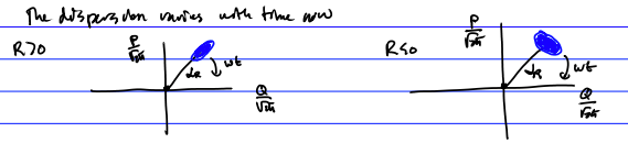
When we have \(R >0\), we have the best accuracy for measuring when the field amplitude is large
When we have \(R < 0\) we have the best accuracy for measuring when the field amplitude is zero.
The latter is best for measuring the phase as where the field crosses zero tells us the phase.
When we measure on a beam splitter the loss is given by \(t < 1, r>0\).

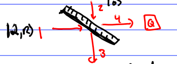
We determine the operator in output port 4: \[\begin{aligned} \hat{Q}_{4}&=\sqrt{\frac{\hbar}{2}}\left(\hat{a}_{4}+\hat{a}_{4}^{\dagger}\right)= \sqrt{\frac{\hbar}{2}}\left(t \hat{a}_{1}-r \hat{a}_{2}+t \hat{a}_{1}^{\dagger}-r\hat{a}_{2}^{\dagger}\right) \\ &= \sqrt{\frac{\hbar}{2}}\left(t\left(\hat{A}_{R} \cosh R-\hat{A}_{R}^{\dagger} \sinh R\right)-r \hat{a}_{2}\right. \\ &\left.+t\left(\hat{A}_{R}^{\dagger} \cosh R-\hat{A}_{R} \sinh R\right)-r \hat{a}_{2}^{\dagger}\right) \\ &= \sqrt{\frac{\hbar}{2}}\left(t \hat{A}_{R} e^{-R}+t \hat{A}_{R}^{\dagger} e^{-R}-r \hat{a}_{2}-r \hat{a}_{2}^{\dagger}\right) \\ &\langle\alpha R| \hat{Q}_{4}|\alpha R\rangle= \sqrt{\frac{\hbar}{2}} t e^{-R}(2 \alpha) \quad \text { for } \alpha \text { real } \\ &\langle\alpha R| \hat{Q}_{4}^{2}|\alpha R\rangle-\left(\langle\alpha R| \hat{Q}_{4}|\alpha R\rangle\right)^{2}=\frac{\hbar}{2}\left(t^{2} e^{-2 R}+\underbrace{r^{2}}_{\text{vac flucs of channel 2}}\right) \\ \end{aligned}\] The vacuum fluctuations from channel 2 can ruin benefits of squeezing when one has losses.
Carlton Caves showed in 1980 how squeezing help one measure on a Mach-Zehnder interferometer. I will give a brief description of how this works, but will not go though the detailed calculations.

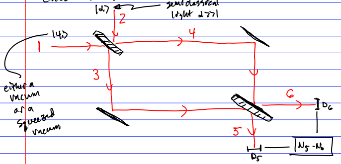
Note how this is essentially a balanced homodyne detection at the lower right. \[\begin{aligned} & \left\langle\psi_{\text {in }}\right| \hat{N}_{5}-\hat{N}_{6}\left|\psi_{\text {in }}\right\rangle=\alpha \sqrt{\frac{2}{\hbar}}\left\langle\psi_{1}\right|\hat{P}_{1}\left|\psi_{1}\right\rangle \\ & \left.\left\langle\psi_{\text {in }}\right|\left(\hat{N}_{5}-\hat{N}_{6}\right)^{2} \mid \psi_{\text {in }}\right.\rangle=\alpha^{2} \frac{2}{\hbar}\left\langle\psi_{1}\right| \hat{P}_{1}^{2}\left|\psi_{1}\right\rangle \end{aligned}\] So the fluctuations are determined by \(\left(\Delta P_{1}\right)_{\psi_1}^{2}\). If we use an ordinary vacuum \(\left(\Delta P_{1}\right)_{\psi_1}^{2}=\frac{\hbar}{2}\), but if we use a "R-squeezed vacuum" \(\left(\Delta P_{1}\right)_{\psi_1}^{2}=\frac{\hbar}{2} e^{2 R}\). So with \(R<0\), we get an improvement.
Note, the squeezed vacuum has photons in it. It is fragile and the gains are reduced by the losses. So one needs super high quality mirrors and optics.
The improvement of accuracy by \(1+\delta\), will increase the volume of observed universe by \((1+\delta)^{3}\). So even small improvements will create huge increases in the observable universe with gravity waves.
LIGO is a similar interferometer.
Gravity waves are quadrupole waves.

Each arm is 4 km long and detects \(\frac{\delta L}{L} \sim 10^{-21}\) or a measurement of \(10^{-18} \mathrm{~m} \quad\) ( \(\frac{1}{1000}\) the radius of a nucleus)!
Resonant cavities are used. These increase the effective length by a factor of 300 . Interferometry can measure \(\sim 10 \mathrm{~nm} \quad (\lambda \sim 500 \mathrm{~nm})\).
So the length difference is \(\frac{\delta L}{L}=\frac{10 \times 10^{-9}\mathrm{~m}}{300 \cdot 4000 \mathrm{~m}} \sim 10^{-14}\).
I believe the other 7 orders of magnitude come from the \(|\alpha|^{2}\) from the lasers, but I have not been ale to confirm this.
The squeezed vacuum reduces noise by \(28 \%\).
\(\Rightarrow(1.28)^{3} \sim\) twice as much universe can be observed!

The squeezed vacuum is used in all gravitational wave detectors now.