Introduction and counting states

Consider the two-site Hubbard model Hamiltonian: \[H = -t \sum_\sigma (c_{1\sigma}^\dagger c_{2\sigma}^{\phantom{\dagger}} + c_{2\sigma}^\dagger c_{1\sigma}^{\phantom{\dagger}}) + U \sum_{i=1}^2 n_{i\uparrow} n_{i\downarrow}\] If there are \(N\) sites, then we claim that there will be \(4^N\) possible states since each site needs to be specified as either \(0, \uparrow, \downarrow, \uparrow\downarrow\), i.e. vacant, one spin up particle, one spin down particle, or two particles with opposite spin. If we have a total of \(m\) electrons (\(0 \leq m \leq 2N\)), the number of states is given by: \[\binom{2N}{m} = \frac{(2N)!}{m!(2N-m)!}\] states with exactly \(m\) electrons. This follows since each electron can be spin-up or spin-down on each site. Hence, there are \(2N\) choices, and we choose \(m\) of them. As a verification, we can check that \[\sum_{m=0}^{2N} \binom{2N}{m} = 2^{2N} = 4^N\] using the binomial theorem and if we choose \(N=2\), then we can count the number of states to be:

• \(m = 0:\) \(\binom{4}{0} = 1\) state.

• \(m = 1:\) \(\binom{4}{1} = 4\) states.

• \(m = 2:\) \(\binom{4}{2} = 6\) states.

• \(m = 3:\) \(\binom{4}{3} = 4\) states.

• \(m = 4:\) \(\binom{4}{4} = 1\) state.

Thus, adding up all states, we get 16 states which equals \(4^N=4^2\). Let’s study each case more specifically.

Energy Eigenstates

1. \(m=0\): \(J = 1, m_J = -1, S= 0\) is the ground state \(|0\rangle\) with energy \(E = 0\)

2. \(m=1\): \(J=1/2, m_J = -1/2, S=1/2\), considering spatial symmetry, this case has two states:

   • \(|1\rangle = \frac{1\uparrow + 2\uparrow}{\sqrt{2}}\) which is shorthand for \(\frac{1}{\sqrt{2}}(c^\dagger_{1\uparrow} |0\rangle +c^\dagger_{2\uparrow} |0\rangle )\)

   • \(|2\rangle = \frac{1\uparrow - 2\uparrow}{\sqrt{2}}\)

   The energies can be found as:

   • \(\hat{T}|1\rangle = -t|1\rangle\), so \(E= -t\). Note that this state has a two fold degeneracy with \(\uparrow\) and \(\downarrow\) cases.

   • \(\hat{T}|2\rangle = t|2\rangle\), so \(E= t\). This state also has a two fold degeneracy as above.

3. \(m=2\):

   1. \(J=1, m_J = 0, S=0\). Here we have \(J^\dagger|0\rangle = \frac{1}{\sqrt{2}}(1\uparrow1\uparrow - 2\uparrow2\uparrow) = |1\rangle\) and \(\hat{T}|1\rangle = -t \frac{1}{\sqrt{2}}(2\uparrow1\downarrow + 1\uparrow2\downarrow - 1\uparrow2\downarrow - 2\uparrow1\downarrow) =0\) and \(\hat{U}|1\rangle = U|1\rangle\) which implies \(E=U\) as it must since \(J^\dagger\) raises \(E\) by \(U\).

   2. \(J=0, m_J = 0, S=1\). Here we have \(1\uparrow2\uparrow = |1\rangle\) and \(H|\uparrow\rangle=0\) so \(E=0\) with a threefold degeneracy.

   3. \(J=0, m_J = 0, S=0\). Here we have two states:

      • \(|1\rangle = \frac{1}{\sqrt{2}} \left( 1\uparrow 1\downarrow + 2\uparrow 2\downarrow \right)\) with \(\hat{H}|1\rangle = -t\frac{1}{\sqrt{2}}(2\uparrow1\downarrow+1\uparrow2\downarrow+1\uparrow2\downarrow+2\uparrow1\downarrow ) + U|1\rangle =-2t|2\rangle+ U |1\rangle\)

      • \(|2\rangle = \frac{1}{\sqrt{2}} \left( |\uparrow \downarrow\rangle - |\downarrow \uparrow\rangle \right)\) with \(\hat{H}|2\rangle = -t\frac{1}{\sqrt{2}}(2\uparrow2\downarrow+1\uparrow1\downarrow+2\downarrow2\uparrow+1\downarrow1\uparrow ) =-2t|1\rangle\)

      Putting the two together, we get: \[H = \begin{pmatrix} U & -2t \\ -2t & 0 \end{pmatrix}\] which has eigenvalues given by \(E^2 - UE - 4t^2 = 0\), which implies: \[E = \frac{U}{2} \pm \frac{1}{2} \sqrt{U^2 + 16t^2}.\]

Summary

Thus, we can summarize the results above in the following table: \[\begin{array}{|c|c|c|c|c|} \hline m & J & S & E & \text{Number of States} \\ \hline 0 & 1 & 0 & E = 0 & 1 \text{ state} \\ 1 & \frac{1}{2} & \frac{1}{2} & E = \pm t \; (\text{twofold}) & 4 \text{ states} \\ 2 & 1 & 0 & E = 0 & 1 \text{ state} \\ & 0 & 1 & E = 0 \; (\text{threefold}) & 3 \text{ states} \\ & 0 & 0 & E = \frac{U}{2} \pm \frac{1}{2} \sqrt{U^2 + 16t^2} & 2 \text{ states} \\ \hline \end{array}\]

Note that the ground state always has the minimal \(J\) and minimal \(S\). In general, one finds minimal \(S\) for \(U<0\) and minimal \(J\) for \(U>0\).

Let us now examine the ground state wavefunction for \(m=2\) as follows: \[\begin{pmatrix} U-\frac{U}{2} + \frac{1}{2} \sqrt{U^2 + 16t^2} & -2t \\ -2t & -\frac{U}{2} + \frac{1}{2} \sqrt{U^2 + 16t^2} \end{pmatrix} \begin{pmatrix} \alpha \\ \beta \end{pmatrix} = 0\] Thus, we get the equation: \[\bigg(\frac{U}{2} + \frac{1}{2} \sqrt{U^2 + 16t^2} \bigg)\alpha - 2t\beta =0\] Rearranging, we get when solving for \(\beta\): \[\beta = \bigg(\frac{U}{4t} + \frac{1}{4t} \sqrt{U^2 + 16t^2} \bigg) \alpha\] Using the normalization \(\alpha^2 + \beta^2 = 1\), we get when substituting in for \(\beta\): \[\alpha^2(1 + \beta^2 ) = \alpha^2\bigg(1 + \bigg(\bigg(\frac{U}{4t} + \frac{1}{4t} \sqrt{U^2 + 16t^2} \bigg) \alpha\bigg)^2 \bigg)= 1\] Expanding out: \[\alpha^2 \left( 1 + \frac{U^2}{16t^2} + \frac{2U}{16t^2} \sqrt{U^2 + 16t^2} + \frac{U^2 + 16t^2}{16t^2} \right) = 1\] and solving for \(\alpha\): \[\alpha = \frac{1}{\sqrt{2\left( 1 + \frac{U^2}{16t^2} + \frac{2U}{16t^2} \sqrt{U^2 + 16t^2} \right)}} = \frac{1}{\sqrt{\frac{2 \sqrt{U^2 + 16t^2}}{16t^2}(U + \sqrt{U^2 + 16t^2})}}\] Hence, \(\beta\) is: \[\beta = \frac{\sqrt{2t} \sqrt{\frac{U}{4t} + \frac{1}{4t} \sqrt{U^2 + 16t^2}}}{(U^2 + 16t^2)^{1/4}}\] Now let the quantum state vector be: \[|\psi\rangle = \alpha |1\rangle + \beta |2\rangle\]

Limiting cases

We can study it in the following limits:

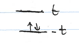
• \(U \to 0\): \(\alpha \to \frac{1}{\sqrt{2}}\), \(\beta \to \frac{1}{\sqrt{2}}\). \[|\psi\rangle \to \frac{1}{\sqrt{2}} \left(|1\rangle + |2\rangle \right) = \frac{1}{2}\left(1\uparrow 1\downarrow + 2\uparrow2\downarrow + 1\uparrow2\downarrow +1\downarrow2\uparrow\right) = \frac{1}{\sqrt{2}}\left(1\uparrow + 2\uparrow \right) \frac{1}{\sqrt{2}}\left(1\downarrow + 2\downarrow \right)\] When \(U=0\), we fill the lowest states of the band structure:

  

• \(U \to \infty\): \(\alpha \to 0\), \(\beta \to 1\). \[|\psi\rangle \to |2\rangle = \frac{1}{\sqrt{2}} \left(1\uparrow 2\downarrow - 1\downarrow2\uparrow \right)\] This state is degenerate with \(\frac{1}{\sqrt{2}} \left(1\uparrow 2\downarrow + 1\downarrow2\uparrow \right), 1\uparrow2\uparrow,\) and \(1\downarrow2\downarrow\) with \(E=0\). When \(U=\infty\), there is no double occupancy so \(E\to 0\). As \(U\to\infty\), all singly occupied states are degenerate as \(U\) decreases and the \(S=0\) state is the lowest.

• \(U \to -\infty\): \(\alpha \to 1\), \(\beta \to 0\). \[|\psi\rangle \to |1\rangle = \frac{1}{\sqrt{2}} \left(1\uparrow 1\downarrow + 2\uparrow2\downarrow \right)\] This state is degenerate with \(\frac{1}{\sqrt{2}} \left(1\uparrow 1\downarrow - 2\uparrow2\downarrow \right)\). As \(U\to-\infty\), only doubly occupied states are allowed. and both degnerate states have \(E=U\to -\infty\)

For the more general cases, we have the following. For \(U =\infty\) at half-filling, all singly occupied states are degenerate. The system is frozen in an insulator. As \(U < \infty\) but large, on a bipartite lattice, the \(S = 0\) state is the lowest in energy. By performing a partial particle-hole transformation \(S \leftrightarrow J\), the ground state for \(U =- \infty\) has all doubly occupied states degenerate. For \(U > -\infty\) but large and negative, on a bipartite lattice, one has \(J = 0\) as the ground state.

In the article, you can learn about other approximations to the ground-state exact solution and see how accurate they are for different \(U\) values. We won’t examine further here.