In quantum mechanics, we define a vector operator via \[\left[\hat{v}_{i}, \hat{L}_{j}\right]=i \hbar \sum_k\varepsilon_{i j k} \hat{v}_{k}\] Oddly, it also satisfies \(\left[\hat{L}_{i}, \hat{v}_{j}\right]=i \hbar \sum_k\varepsilon_{i j k} \hat{v}_{k}\) as well. One might have thought there is a sign change, but there isn’t. On the homework, you will verify that \(\hat{\mathbf{r}}\) and \(\hat{\mathbf{p}}\) are both vector operators.
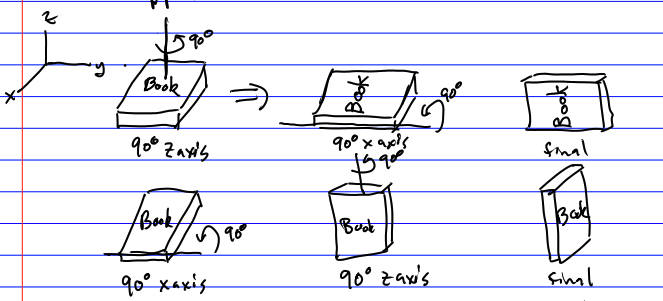
Let’s start with rotations. First note that rotations form a group (closed under multiplication, unique inverse, etc.). But they are a non-Abelian group, because when we apply the rotations in one order, they are not the same as when we apply them in the opposite order:
The claim is all rotations can be written as \[\hat{R}\left(\alpha, \mathbf{e}_{n}\right)=\exp \left[-i \frac{\alpha}{\hbar} \mathbf{e}_{n} \cdot \hat{\mathbf{L}}\right]\] \(\mathbf{e}_{n}\), a unit vector, is the axis of the rotation and \(\alpha\) is the angle of the rotation in radians. \(\hat{\mathbf{L}}\) is the quantum operator for angular momentum. If you look back to what we did with the spin matrices in lecture 1, we showed this holds there as well with \(\hat{\mathbf{L}} \rightarrow \hat{\mathbf{S}}=\frac{\hbar}{2} \mathbf{\sigma}\). (The factor of \(\frac{1}{2}\) is needed to be correct).
Suppose we transform states via \(|\psi\rangle \rightarrow \hat{R}|\psi\rangle\), then \(\hat{O}|\psi\rangle \rightarrow \hat{R} \hat{O}|\psi\rangle=\hat{R} \hat{O} \hat{R}^{\dagger}(\hat{R}|\psi\rangle)\). This implies that operators transform as \(\hat{O} \rightarrow \hat{R} \hat{O} \hat{R}^{\dagger}\).
On the HW, we showed that \[\begin{aligned} & \hat{R}\left(\alpha, \hat{e}_{z}\right) \hat{L}_{z} \hat{R}^{\dagger}\left(\alpha, \hat{e}_{z}\right)=\hat{L}_{z} \\ & \hat{R}\left(\alpha, \hat{e}_{z}\right) \hat{L}_{x} \hat{R}^{\dagger}\left(\alpha, \hat{e}_{z}\right)=\cos \alpha \hat{L}_{x}+\sin \alpha \hat{L}_{y} \\ & \hat{R}\left(\alpha, \mathbf{e}_{z}\right) \hat{L}_{y} \hat{R}^{\dagger}\left(\alpha, \hat{e}_{z}\right)=-\sin \alpha \hat{L}_{x}+\cos \alpha \hat{L}_{y} \end{aligned}\] We did this by using the Hadamard identity. This is an easier way to do the calculation than to use disentangling. Since a vector operator satisfies the same commutation with \(\hat{\mathbf{L}}\) as \(\hat{\mathbf{L}}\) does (i.e. \(\hat{\mathbf{L}}\) is a vector operator), we have \[\begin{aligned} & e^{-i \alpha \frac{\hat{L}_{z}}{\hbar}} \hat{v}_{i} e^{i \alpha \frac{\hat{L}_{z}}{\hbar}}=\sum_{j} O_{i j}^{(z)} \hat{v}_{j} \\ & O^{(z)}=\left(\begin{array}{ccc} \cos \alpha & \sin \alpha & 0 \\ -\sin \alpha & \cos \alpha & 0 \\ 0 & 0 & 1 \end{array}\right) \end{aligned}\]
Next, via permutations, we can verify that \[\begin{aligned} & e^{-i \alpha \frac{\hat{L}_{x}}{\hbar}} \hat{v}_{i} e^{i \alpha \frac{\hat{L}_{x}}{\hbar}}=\sum_{j} O_{i j}^{(x)} \hat{v}_{j} \\ & e^{-i \alpha \frac{\hat{L}_{y}}{\hbar}} \hat{v}_{i} e^{i \alpha \frac{\hat{L}_{y}}{\hbar}}=\sum_{j} O_{i j}^{(y)} \hat{v}_{j} \\ & \hat{O}^{(x)}=\left(\begin{array}{ccc} 1 & 0 & 0 \\ 0 & \cos \alpha & \sin \alpha \\ 0 & -\sin \alpha & \cos \alpha \end{array}\right) \quad \hat{O}^{(y)}=\left(\begin{array}{ccc} \cos \alpha & 0 & -\sin \alpha \\ 0 & 1 & 0 \\ \sin \alpha & 0 & \cos \alpha \end{array}\right) \end{aligned}\]
What about the general case \(e^{-i \alpha \frac{\mathbf{e}_{n} \cdot \hat{\mathbf{L} }}{\hbar}}\)? We can work this out with no extra calculation using only geometry. Assume \(\mathbf{e}_{n}\) points in the \(\theta , \phi\) direction.
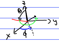
The spherical unit vectors are \[\begin{aligned} & \mathbf{e}_{n}=\left(\sin \theta \cos \phi, \sin \theta \sin \phi, \cos \theta\right) \\ & \mathbf{e}_{\theta}=\left(\cos \theta \cos \phi, \cos \theta \sin \phi,-\sin \theta\right) \\ & \mathbf{e}_{\phi}=\left(-\sin \phi, \cos \phi , 0\right) \end{aligned}\]
We can use the results we already calculated, assuming we can establish they hold in the new \(n, \theta, \phi\) coordinate system. That is, if \(\beta \in\{n, \theta, \phi\}\), we need to show \[\left[\hat{L}_{\beta}, \hat{v}_{\gamma}\right]=i \hbar \sum_\delta\varepsilon_{\beta \gamma \delta} \hat{v}_{\delta}\]
Consider the orthogonal matrix \(O\) that satisfies \[\begin{aligned} & \mathbf{e}_{n}= O \mathbf{e}_{z} \\ & \mathbf{e}_{\theta}=O \mathbf{e}_{x} \\ & \mathbf{e}_{\phi}=O \mathbf{e}_{y} \end{aligned}\]
From the results we found for \(\mathbf{e}_{n}, \mathbf{e}_{\theta}\) and \(\mathbf{e}_{\phi}\), we have \[O=\left(\begin{array}{ccc} \cos \theta \cos \phi & -\sin \phi & \sin \theta \cos \phi \\ \cos \theta \sin \phi & \cos \phi & \sin \theta \sin \phi \\ -\sin \theta & 0 & \cos \theta \end{array}\right),\] but we really only need the fact that \(O^{T} O=1\) which implies that \(O\) is orthogonal.
Note, we have \(v_{\beta}=\sum_{j} O_{i j} v_{j}\) with
| \(\beta\) | \(i\) | |
| \(n\) | \(\leftrightarrow\) | \(z\) |
| \(\theta\) | \(\leftrightarrow\) | \(x\) |
| \(\phi\) | \(\leftrightarrow\) | \(y\) |
The commutation relation is \[\begin{aligned} & {\left[\hat{v}_{\beta,} \hat{L}_{\gamma}\right]=i \hbar O_{ii^{\prime}} O_{jj^{\prime}} \varepsilon_{i^{\prime} j^{\prime} k^{\prime}} \underbrace{\hat{v}_{k^{\prime}}}_{\text{Cartesian basis}}} \end{aligned}\] Here we have \(\beta \leftrightarrow i \quad \gamma \leftrightarrow j\) and repeated indices are summed over. But, \[v_{k^{\prime}}=O_{k^{\prime} \delta}^{T} O_{\delta l} \hat{v}_{l} = i \hbar \varepsilon_{i^{\prime} j^{\prime} k^{\prime}} O_{i i^{\prime}} O_{j j^{\prime}} \underbrace{O_{\delta k^{\prime}} \hat{v}_{\delta}}_{\text{spherical}} .\] If \(\sum_{i^{\prime} j^{\prime} k^{\prime}} \varepsilon_{i^{\prime} j^{\prime} k^{\prime}} O_{i i^{\prime}} O_{j j^{\prime}} O_{k k^{\prime}}=\underbrace{\varepsilon_{i j k}}_{\text {spherical}}\), then we have \([\hat{v}_{\beta},\hat{L}_{\gamma}] = i \hbar \varepsilon_{\beta \gamma \delta } \hat{v}_\delta\) in the spherical basis.
Check: \(i=j=n \quad
\underbrace{\varepsilon_{i^{\prime} j^{\prime}
k^{\prime}}}_{\text{anti-symmetric on interchange of } i^{\prime}
j^{\prime}} \underbrace{O_{n i^{\prime}} O_{k
j^{\prime}}}_{\text{symmetric on interchange of } i^{\prime} j^{\prime}}
O_{k k^{\prime}} \Rightarrow O\)
\[\begin{aligned}
& i=n, j=\theta: \\
& \Rightarrow \varepsilon_{x y z} O_{n x} O_{\theta y} O_{\delta
z}+\varepsilon_{y z x} O_{n y} O_{\theta z} O_{\delta x}+\varepsilon_{z
x y} O_{n z} O_{\theta x} O_{\delta y} \\
&+\varepsilon_{x z y} O_{n x} O_{\theta z} O_{\delta
y}+\varepsilon_{z y x} O_{n z} O_{\theta y} O_{\delta x}+\varepsilon_{y
x z} O_{n y} O_{\theta x} O_{\delta z}
\end{aligned}\] The top row has all \(\varepsilon\)’s \(+1\), bottom has all \(-1\). Careful inspection shows this is
\(\operatorname{det} O\). But since
\(O^{T} O=\mathbb{I} \Rightarrow
\operatorname{det} O^{T} \operatorname{det} O=1 \Rightarrow
\operatorname{det} O= \pm 1\) for rotations, we find \(\operatorname{det} O=1\) (just calculate
the determinant of the explicit matrix \(O\) above).
It is easy to see from this that we have established the result we need. Essentially we have after the rotation \(\mathbf{e}_{z} \rightarrow \mathbf{e}_{n} \quad \mathbf{e}_{x} \rightarrow \mathbf{e}_{\theta} \quad \mathbf{e}_{y} \rightarrow \mathbf{e}_{\phi}\).
You should have already verified from the algebras of \(\hat{L}_{x}, \hat{L}_{y}\) and \(\hat{L}_{z}\) that
\[\begin{aligned} \hat{L}_{z}|l m\rangle & =\hbar m|l m\rangle \\ \hat{L}_{+}|l m\rangle & =\hbar \sqrt{l(l+1)-m(m+1)} | l m+1) \\ & =\hbar \sqrt{(l-m)(l+m+1)}|l m+1\rangle \\ \hat{L}_{-}|l m\rangle & =\hbar \sqrt{l(l+1)-m(m-1)}|l m-1\rangle \\ & =\hbar \sqrt{(l+m)(l-m+1)}|l m-1\rangle \\ \hat{L}^{2}|l m\rangle & =\hbar^{2} l(l+1)|l m\rangle \end{aligned}\] Using \(\hat{L}^{2}=\frac{1}{2}\left(\hat{L}_{+} \hat{L}_{-}+\hat{L}_{-} \hat{L}_{+}\right)+\hat{L}_{z} \hat{L}_{z}\) and the above results we see that because \[\begin{aligned} \frac{\hbar^{2}}{2} & {[\sqrt{(l-m)(l+m+1)} \sqrt{(l+m+1)(l-m)}} \\ & +\sqrt{(l+m)(l-m+1)(l-m+1)(l+m)}]+\hbar^{2} m^{2} \\ = & \hbar^{2}\left[\frac{1}{2}(l-m)(l+m+1)+\frac{1}{2}(l+m)(l-m+1)+m^{2}\right] \\ & =\hbar^{2}\left[\frac{1}{2}\left(l^{2}-m^{2}+l-m+l^{2}-m^{2}+l+m\right)+m^{2}\right] \\ & =\hbar^{2} l(l+1). \end{aligned}\]
We can put these results together to verify that \[|\theta, \phi\rangle=e^{-i \phi \frac{\hat{L}_{z}}{\hbar}} e^{-i \theta \frac{\hat{L}_{y}}{\hbar}}|\theta{=}0, \phi{=}0\rangle.\]
As a check, we verify that \[\begin{aligned} & e^{i \hat{\theta}}|\theta, \phi\rangle=e^{i \theta}|\theta, \phi\rangle \\ & e^{i \hat{\phi}}|\theta, \phi\rangle=e^{i \phi}|\theta, \phi\rangle \end{aligned}\] with \(e^{i \hat{\theta}}=\frac{\hat{z}+i \sqrt{\hat{x}^{2}+\hat{y}^{2}}}{\hat{r}} \quad e^{i \hat{\phi}}=\frac{\hat{x}+i \hat{y}}{\sqrt{\hat{x}^{2}+\hat{y}^{2}}}\). We must define these in this way because \(\hat{\theta}\) and \(\hat{\phi}\) are not well-defined quantum operators.
Because \(\hat{r}\) commutes with \(\hat{\mathbf{L}}\) and \((\hat{x}, \hat{y}, \hat{z})\) is a vector operator, we can establish this result via Hadamard. You will verify this on the homework.
We end by discussing exponential disentangling. We will need to
compute \[e^{i \theta
\frac{\hat{L}_{y}}{\hbar}}=e^{i \frac{\theta}{\hbar}
\frac{\hat{L}_{+}-\hat{L}_{-}}{2i}} =e^{\frac{\theta}{2
\hbar}\left(\hat{L}_{+}-\hat{L}_{-}\right)}\] We derived
disentangling in lecture 1. It gives \[e^{\frac{\theta}{2
\hbar}(\hat{L}_{+}-\hat{L}_{-})}=e^{-\tan \left(\frac{\theta}{2}\right)
\frac{\hat{L}_{-}}{\hbar}-} e^{2 \ln \cos \frac{\theta}{2}
\frac{\hat{L}_{z}}{\hbar}} e^{\tan \left(\frac{\theta}{2}\right)
\frac{\hat{L}_{z}}{\hbar}}\] (there is a similar one with \(\hat{L}_{-}\) on the right and \(\hat{L}_{+}\)on the left)
We will use this to find spherical harmonics in the next lecture. In
particular, note that \[\begin{aligned}
\left|\theta , \phi\right\rangle & =e^{-i \phi
\frac{\hat{L}_{z}}{\hbar}} e^{-i \frac{\theta
\hat{L}_{y}}{\hbar}}|\theta{=}0, \phi{=}0\rangle \\
& =e^{-i \phi \frac{\hat{L}_{z}}{\hbar}} e^{\tan
\left(\frac{\theta}{2}\right) \frac{\hat{L}_{-}}{\hbar}} e^{2 \ln \cos
\frac{\theta}{2} \frac{\hat{L}_{z}}{\hbar}} e^{-\tan
\left(\frac{\theta}{2}\right) \frac{\hat{L}_{+}}{\hbar}} | \theta{=}0,
\phi{=}0 \rangle
\end{aligned}\] At the moment this does not look too exciting,
but we will see that it is exactly what we need in the next lecture.